Closeness Centrality

This section describes the Closeness Centrality algorithm in the Neo4j Graph Data Science library.

Closeness centrality is a way of detecting nodes that are able to spread information very efficiently through a graph.

The closeness centrality of a node measures its average farness (inverse distance) to all other nodes. Nodes with a high closeness score have the shortest distances to all other nodes.

This algorithm is in the alpha tier. For more information on algorithm tiers, see Algorithms.

1. History and explanation

For each node u, the Closeness Centrality algorithm calculates the sum of its distances to all other nodes, based on calculating the shortest paths between all pairs of nodes. The resulting sum is then inverted to determine the closeness centrality score for that node.

The raw closeness centrality of a node u is calculated using the following formula:

raw closeness centrality(u) = 1 / sum(distance from u to all other nodes)

It is more common to normalize this score so that it represents the average length of the shortest paths rather than their sum. This adjustment allow comparisons of the closeness centrality of nodes of graphs of different sizes

The formula for normalized closeness centrality of node u is as follows:

normalized closeness centrality(u) = (number of nodes - 1) / sum(distance from u to all other nodes)

 Wasserman and Faust have proposed an improved formula for dealing with unconnected graphs.
Assuming that _n_  is the number of nodes reachable from _u_ (counting also itself),
their corrected formula for a given node _u_ is given as follows

Wasserman-Faust normalized closeness centrality(u) = (n-1)^2/ number of nodes - 1) * sum(distance from u to all other nodes

Note that in the case of a directed graph, closeness centrality is defined alternatively. That is, rather than considering distances from u to every other node, we instead sum and average the distance from every other node to u.

2. Use-cases - when to use the Closeness Centrality algorithm

Closeness centrality is used to research organizational networks, where individuals with high closeness centrality are in a favourable position to control and acquire vital information and resources within the organization. One such study is "Mapping Networks of Terrorist Cells" by Valdis E. Krebs.
Closeness centrality can be interpreted as an estimated time of arrival of information flowing through telecommunications or package delivery networks where information flows through shortest paths to a predefined target. It can also be used in networks where information spreads through all shortest paths simultaneously, such as infection spreading through a social network. Find more details in "Centrality and network flow" by Stephen P. Borgatti.
Closeness centrality has been used to estimate the importance of words in a document, based on a graph-based keyphrase extraction process. This process is described by Florian Boudin in "A Comparison of Centrality Measures for Graph-Based Keyphrase Extraction".

3. Constraints - when not to use the Closeness Centrality algorithm

Academically, closeness centrality works best on connected graphs. If we use the original formula on an unconnected graph, we can end up with an infinite distance between two nodes in separate connected components. This means that we’ll end up with an infinite closeness centrality score when we sum up all the distances from that node.

In practice, a variation on the original formula is used so that we don’t run into these issues.

4. Syntax

The following will run the algorithm and write back results:

CALL gds.alpha.closeness.write(configuration: Map)
YIELD nodes, createMillis, computeMillis, writeMillis, centralityDistribution

Table 1. Parameters
Name	Type	Default	Optional	Description
concurrency	int	4	yes	The number of concurrent threads used for running the algorithm. Also provides the default value for 'readConcurrency' and 'writeConcurrency'.
readConcurrency	int	value of 'concurrency'	yes	The number of concurrent threads used for reading the graph.
writeConcurrency	int	value of 'concurrency'	yes	The number of concurrent threads used for writing the result.
writeProperty	string	'centrality'	yes	The property name written back to.
improved	boolean	false	yes	Denotes whether the Wasserman-Faust formula is used.

Table 2. Results
Name	Type	Description
nodes	int	The number of nodes considered.
createMillis	int	Milliseconds for loading data.
computeMillis	int	Milliseconds for running the algorithm.
writeMillis	int	Milliseconds for writing result data back.
writeProperty	string	The property name written back to.
centralityDistribution	Map	Map containing min, max, mean as well as p50, p75, p90, p95, p99 and p999 percentile values of centrality values.

The following will run the algorithm and stream results:

CALL gds.alpha.closeness.stream(configuration: Map)
YIELD nodeId, centrality

Table 3. Parameters
Name	Type	Default	Optional	Description
concurrency	int	4	yes	The number of concurrent threads used for running the algorithm. Also provides the default value for 'readConcurrency' and 'writeConcurrency'.
readConcurrency	int	value of 'concurrency'	yes	The number of concurrent threads used for reading the graph.

Table 4. Results
Name	Type	Description
node	long	Node ID
centrality	float	Closeness centrality score

5. Closeness Centrality algorithm sample

The following will create a sample graph:

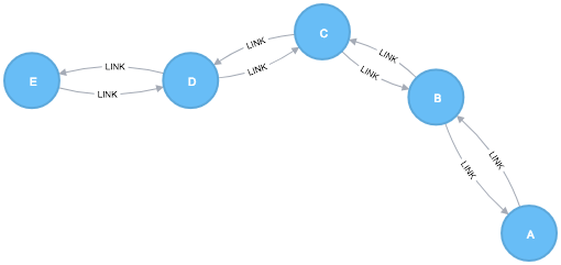
CREATE (a:Node{id:"A"}),
       (b:Node{id:"B"}),
       (c:Node{id:"C"}),
       (d:Node{id:"D"}),
       (e:Node{id:"E"}),
       (a)-[:LINK]->(b),
       (b)-[:LINK]->(a),
       (b)-[:LINK]->(c),
       (c)-[:LINK]->(b),
       (c)-[:LINK]->(d),
       (d)-[:LINK]->(c),
       (d)-[:LINK]->(e),
       (e)-[:LINK]->(d);

The following will run the algorithm and stream results:

CALL gds.alpha.closeness.stream({
  nodeProjection: 'Node',
  relationshipProjection: 'LINK'
})
YIELD nodeId, centrality
RETURN gds.util.asNode(nodeId).name AS user, centrality
ORDER BY centrality DESC

Table 5. Results
Name	Centrality weight
C	0.6666666666666666
B	0.5714285714285714
D	0.5714285714285714
A	0.4
E	0.4

C is the best connected node in this graph, although B and D aren’t far behind. A and E don’t have close ties to many other nodes, so their scores are lower. Any node that has a direct connection to all other nodes would score 1.

The following will run the algorithm and write back results:

CALL gds.alpha.closeness.write({
  nodeProjection: 'Node',
  relationshipProjection: 'LINK',
  writeProperty: 'centrality'
}) YIELD nodes, writeProperty

Table 6. Results
nodes	writeProperty
5	"centrality"

6. Cypher projection

If node labels and relationship types are not selective enough to project a graph, you can use Cypher queries instead. Cypher projections can also be used to run algorithms on a virtual graph. You can learn more in the Creating graphs using Cypher section of the manual.

CALL gds.alpha.closeness.write({
  nodeQuery: 'MATCH (p:Node) RETURN id(p) AS id',
  relationshipQuery: 'MATCH (p1:Node)-[:LINK]->(p2:Node) RETURN id(p1) AS source, id(p2) AS target'
}) YIELD nodes, writeProperty

Table 7. Results
nodes	writeProperty
5	"centrality"

Calculation:

count farness in each msbfs-callback
divide by N-1

N = 5 // number of nodes

k = N-1 = 4 // used for normalization

     A     B     C     D     E
 --|-----------------------------
 A | 0     1     2     3     4       // farness between each pair of nodes
 B | 1     0     1     2     3
 C | 2     1     0     1     2
 D | 3     2     1     0     1
 E | 4     3     2     1     0
 --|-----------------------------
 S | 10    7     6     7     10      // raw closeness centrality
 ==|=============================
k/S| 0.4  0.57  0.67  0.57   0.4     // normalized closeness centrality

Was this page helpful?