Local Clustering Coefficient
Glossary
- Directed
-
Directed trait. The algorithm is well-defined on a directed graph.
- Directed
-
Directed trait. The algorithm ignores the direction of the graph.
- Directed
-
Directed trait. The algorithm does not run on a directed graph.
- Undirected
-
Undirected trait. The algorithm is well-defined on an undirected graph.
- Undirected
-
Undirected trait. The algorithm ignores the undirectedness of the graph.
- Heterogeneous nodes
-
Heterogeneous nodes fully supported. The algorithm has the ability to distinguish between nodes of different types.
- Heterogeneous nodes
-
Heterogeneous nodes allowed. The algorithm treats all selected nodes similarly regardless of their label.
- Heterogeneous relationships
-
Heterogeneous relationships fully supported. The algorithm has the ability to distinguish between relationships of different types.
- Heterogeneous relationships
-
Heterogeneous relationships allowed. The algorithm treats all selected relationships similarly regardless of their type.
- Weighted relationships
-
Weighted trait. The algorithm supports a relationship property to be used as weight, specified via the relationshipWeightProperty configuration parameter.
- Weighted relationships
-
Weighted trait. The algorithm treats each relationship as equally important, discarding the value of any relationship weight.
- Node properties
-
Node properties trait. The algorithm makes use of node properties.
Introduction
The Local Clustering Coefficient algorithm computes the local clustering coefficient for each node in the graph. The local clustering coefficient Cn of a node n describes the likelihood that the neighbours of n are also connected. To compute Cn we use the number of triangles a node is a part of Tn, and the degree of the node dn. The formula to compute the local clustering coefficient is as follows:

As we can see the triangle count is required to compute the local clustering coefficient. To do this the Triangle Count algorithm is utilised.
Additionally, the algorithm can compute the average clustering coefficient for the whole graph. This is the normalised sum over all the local clustering coefficients.
For more information, see Clustering Coefficient.
Syntax
This section covers the syntax used to execute the Local Clustering Coefficient algorithm in each of its execution modes. We are describing the named graph variant of the syntax. To learn more about general syntax variants, see Syntax overview.
CALL gds.localClusteringCoefficient.stream(
  graphName: String,
  configuration: Map
)
YIELD
  nodeId: Integer,
localClusteringCoefficient: Double| Name | Type | Default | Optional | Description |
|---|---|---|---|---|
graphName |
String |
|
no |
The name of a graph stored in the catalog. |
configuration |
Map |
|
yes |
Configuration for algorithm-specifics and/or graph filtering. |
| Name | Type | Default | Optional | Description |
|---|---|---|---|---|
List of String |
|
yes |
Filter the named graph using the given node labels. Nodes with any of the given labels will be included. |
|
List of String |
|
yes |
Filter the named graph using the given relationship types. Relationships with any of the given types will be included. |
|
Integer |
|
yes |
The number of concurrent threads used for running the algorithm. |
|
String |
|
yes |
An ID that can be provided to more easily track the algorithm’s progress. |
|
Boolean |
|
yes |
If disabled the progress percentage will not be logged. |
|
triangleCountProperty |
String |
|
yes |
Node property that contains pre-computed triangle count. |
1. In a GDS Session, the default is the number of available processors. |
||||
| Name | Type | Description |
|---|---|---|
nodeId |
Integer |
Node ID. |
localClusteringCoefficient |
Double |
Local clustering coefficient. |
CALL gds.localClusteringCoefficient.stats(
  graphName: String,
  configuration: Map
)
YIELD
  averageClusteringCoefficient: Double,
  nodeCount: Integer,
  preProcessingMillis: Integer,
  computeMillis: Integer,
  postProcessingMillis: Integer,
configuration: Map| Name | Type | Default | Optional | Description |
|---|---|---|---|---|
graphName |
String |
|
no |
The name of a graph stored in the catalog. |
configuration |
Map |
|
yes |
Configuration for algorithm-specifics and/or graph filtering. |
| Name | Type | Default | Optional | Description |
|---|---|---|---|---|
List of String |
|
yes |
Filter the named graph using the given node labels. Nodes with any of the given labels will be included. |
|
List of String |
|
yes |
Filter the named graph using the given relationship types. Relationships with any of the given types will be included. |
|
Integer |
|
yes |
The number of concurrent threads used for running the algorithm. |
|
String |
|
yes |
An ID that can be provided to more easily track the algorithm’s progress. |
|
Boolean |
|
yes |
If disabled the progress percentage will not be logged. |
|
triangleCountProperty |
String |
|
yes |
Node property that contains pre-computed triangle count. |
2. In a GDS Session, the default is the number of available processors. |
||||
| Name | Type | Description |
|---|---|---|
averageClusteringCoefficient |
Double |
The average clustering coefficient. |
nodeCount |
Integer |
Number of nodes in the graph. |
preProcessingMillis |
Integer |
Milliseconds for preprocessing the graph. |
computeMillis |
Integer |
Milliseconds for running the algorithm. |
postProcessingMillis |
Integer |
Milliseconds for computing the global metrics. |
configuration |
Map |
The configuration used for running the algorithm. |
CALL gds.localClusteringCoefficient.mutate(
  graphName: String,
  configuration: Map
)
YIELD
  averageClusteringCoefficient: Double,
  nodeCount: Integer,
  nodePropertiesWritten: Integer,
  preProcessingMillis: Integer,
  computeMillis: Integer,
  postProcessingMillis: Integer,
  mutateMillis: Integer,
configuration: Map| Name | Type | Default | Optional | Description |
|---|---|---|---|---|
graphName |
String |
|
no |
The name of a graph stored in the catalog. |
configuration |
Map |
|
yes |
Configuration for algorithm-specifics and/or graph filtering. |
| Name | Type | Default | Optional | Description |
|---|---|---|---|---|
mutateProperty |
String |
|
no |
The node property in the GDS graph to which the local clustering coefficient is written. |
List of String |
|
yes |
Filter the named graph using the given node labels. |
|
List of String |
|
yes |
Filter the named graph using the given relationship types. |
|
Integer |
|
yes |
The number of concurrent threads used for running the algorithm. |
|
Boolean |
|
yes |
If disabled the progress percentage will not be logged. |
|
String |
|
yes |
An ID that can be provided to more easily track the algorithm’s progress. |
|
triangleCountProperty |
String |
|
yes |
Node property that contains pre-computed triangle count. |
| Name | Type | Description |
|---|---|---|
averageClusteringCoefficient |
Double |
The average clustering coefficient. |
nodeCount |
Integer |
Number of nodes in the graph. |
nodePropertiesWritten |
Integer |
Number of properties added to the projected graph. |
preProcessingMillis |
Integer |
Milliseconds for preprocessing the graph. |
computeMillis |
Integer |
Milliseconds for running the algorithm. |
postProcessingMillis |
Integer |
Milliseconds for computing the global metrics. |
mutateMillis |
Integer |
Milliseconds for adding properties to the projected graph. |
configuration |
Map |
The configuration used for running the algorithm. |
CALL gds.localClusteringCoefficient.write(
  graphName: String,
  configuration: Map
)
YIELD
  averageClusteringCoefficient: Double,
  nodeCount: Integer,
  nodePropertiesWritten: Integer,
  preProcessingMillis: Integer,
  computeMillis: Integer,
  postProcessingMillis: Integer,
  writeMillis: Integer,
configuration: Map| Name | Type | Default | Optional | Description |
|---|---|---|---|---|
graphName |
String |
|
no |
The name of a graph stored in the catalog. |
configuration |
Map |
|
yes |
Configuration for algorithm-specifics and/or graph filtering. |
| Name | Type | Default | Optional | Description |
|---|---|---|---|---|
List of String |
|
yes |
Filter the named graph using the given node labels. Nodes with any of the given labels will be included. |
|
List of String |
|
yes |
Filter the named graph using the given relationship types. Relationships with any of the given types will be included. |
|
Integer |
|
yes |
The number of concurrent threads used for running the algorithm. |
|
String |
|
yes |
An ID that can be provided to more easily track the algorithm’s progress. |
|
Boolean |
|
yes |
If disabled the progress percentage will not be logged. |
|
Integer |
|
yes |
The number of concurrent threads used for writing the result to Neo4j. |
|
String |
|
no |
The node property in the Neo4j database to which the local clustering coefficient is written. |
|
triangleCountProperty |
String |
|
yes |
Node property that contains pre-computed triangle count. |
3. In a GDS Session, the default is the number of available processors. |
||||
| Name | Type | Description |
|---|---|---|
averageClusteringCoefficient |
Double |
The average clustering coefficient. |
nodeCount |
Integer |
Number of nodes in the graph. |
nodePropertiesWritten |
Integer |
Number of properties written to Neo4j. |
preProcessingMillis |
Integer |
Milliseconds for preprocessing the graph. |
computeMillis |
Integer |
Milliseconds for running the algorithm. |
postProcessingMillis |
Integer |
Milliseconds for computing the global metrics. |
writeMillis |
Integer |
Milliseconds for writing results back to Neo4j. |
configuration |
Map |
The configuration used for running the algorithm. |
Examples
|
All the examples below should be run in an empty database. The examples use Cypher projections as the norm. Native projections will be deprecated in a future release. |
In this section we will show examples of running the Local Clustering Coefficient algorithm on a concrete graph. The intention is to illustrate what the results look like and to provide a guide in how to make use of the algorithm in a real setting. We will do this on a small social network graph of a handful nodes connected in a particular pattern. The example graph looks like this:
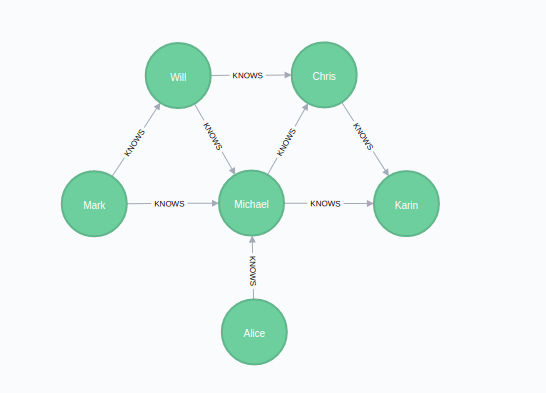
CREATE
  (alice:Person {name: 'Alice'}),
  (michael:Person {name: 'Michael'}),
  (karin:Person {name: 'Karin'}),
  (chris:Person {name: 'Chris'}),
  (will:Person {name: 'Will'}),
  (mark:Person {name: 'Mark'}),

  (michael)-[:KNOWS]->(karin),
  (michael)-[:KNOWS]->(chris),
  (will)-[:KNOWS]->(michael),
  (mark)-[:KNOWS]->(michael),
  (mark)-[:KNOWS]->(will),
  (alice)-[:KNOWS]->(michael),
  (will)-[:KNOWS]->(chris),
  (chris)-[:KNOWS]->(karin)
With the graph in Neo4j we can now project it into the graph catalog to prepare it for algorithm execution.
We do this using a Cypher projection targeting the Person nodes and the KNOWS relationships.
For the relationships we must use the UNDIRECTED orientation.
This is because the Local Clustering Coefficient algorithm is defined only for undirected graphs.
MATCH (source:Person)-[r:KNOWS]->(target:Person)
RETURN gds.graph.project(
  'myGraph',
  source,
  target,
  {},
  { undirectedRelationshipTypes: ['*'] }
)
The Local Clustering Coefficient algorithm requires the graph to use the UNDIRECTED orientation for relationships.
You can either create the graph with undirected relationships or update it by converting the directed relationships into new undirected ones.
|
In the following examples we will demonstrate using the Local Clustering Coefficient algorithm on 'myGraph'.
Memory Estimation
First off, we will estimate the cost of running the algorithm using the estimate procedure.
This can be done with any execution mode.
We will use the write mode in this example.
Estimating the algorithm is useful to understand the memory impact that running the algorithm on your graph will have.
When you later actually run the algorithm in one of the execution modes the system will perform an estimation.
If the estimation shows that there is a very high probability of the execution going over its memory limitations, the execution is prohibited.
To read more about this, see Automatic estimation and execution blocking.
For more details on estimate in general, see Memory Estimation.
CALL gds.localClusteringCoefficient.write.estimate('myGraph', {
  writeProperty: 'localClusteringCoefficient'
})
YIELD nodeCount, relationshipCount, bytesMin, bytesMax, requiredMemory| nodeCount | relationshipCount | bytesMin | bytesMax | requiredMemory |
|---|---|---|---|---|
6 |
16 |
304 |
304 |
"304 Bytes" |
Note that the relationship count is 16 although we only created 8 relationships in the original Cypher statement.
This is because we used the UNDIRECTED orientation, which will project each relationship in each direction, effectively doubling the number of relationships.
Stream
In the stream execution mode, the algorithm returns the local clustering coefficient for each node.
This allows us to inspect the results directly or post-process them in Cypher without any side effects.
For example, we can order the results to find the nodes with the highest local clustering coefficient.
For more details on the stream mode in general, see Stream.
stream mode:CALL gds.localClusteringCoefficient.stream('myGraph')
YIELD nodeId, localClusteringCoefficient
RETURN gds.util.asNode(nodeId).name AS name, localClusteringCoefficient
ORDER BY localClusteringCoefficient DESC, name| name | localClusteringCoefficient |
|---|---|
"Karin" |
1.0 |
"Mark" |
1.0 |
"Chris" |
0.6666666666666666 |
"Will" |
0.6666666666666666 |
"Michael" |
0.3 |
"Alice" |
0.0 |
From the results we can see that the nodes 'Karin' and 'Mark' have the highest local clustering coefficients. This shows that they are the best at introducing their friends - all the people who know them, know each other! This can be verified in the example graph.
Stats
In the stats execution mode, the algorithm returns a single row containing a summary of the algorithm result.
The summary result contains the avearage clustering coefficient of the graph, which is the normalised sum over all local clustering coefficients.
This execution mode does not have any side effects.
It can be useful for evaluating algorithm performance by inspecting the computeMillis return item.
In the examples below we will omit returning the timings.
The full signature of the procedure can be found in the syntax section.
For more details on the stats mode in general, see Stats.
stats mode:CALL gds.localClusteringCoefficient.stats('myGraph')
YIELD averageClusteringCoefficient, nodeCount| averageClusteringCoefficient | nodeCount |
|---|---|
0.6055555555555555 |
6 |
The result shows that on average each node of our example graph has approximately 60% of its neighbours connected.
Mutate
The mutate execution mode extends the stats mode with an important side effect: updating the named graph with a new node property containing the local clustering coefficient for that node.
The name of the new property is specified using the mandatory configuration parameter mutateProperty.
The result is a single summary row, similar to stats, but with some additional metrics.
The mutate mode is especially useful when multiple algorithms are used in conjunction.
For more details on the mutate mode in general, see Mutate.
mutate mode:CALL gds.localClusteringCoefficient.mutate('myGraph', {
mutateProperty: 'localClusteringCoefficient'
})
YIELD averageClusteringCoefficient, nodeCount| averageClusteringCoefficient | nodeCount |
|---|---|
0.6055555555555555 |
6 |
The returned result is the same as in the stats example.
Additionally, the graph 'myGraph' now has a node property localClusteringCoefficient which stores the local clustering coefficient for each node.
To find out how to inspect the new schema of the in-memory graph, see Listing graphs.
Write
The write execution mode extends the stats mode with an important side effect: writing the local clustering coefficient for each node as a property to the Neo4j database.
The name of the new property is specified using the mandatory configuration parameter writeProperty.
The result is a single summary row, similar to stats, but with some additional metrics.
The write mode enables directly persisting the results to the database.
For more details on the write mode in general, see Write.
write mode:CALL gds.localClusteringCoefficient.write('myGraph', {
writeProperty: 'localClusteringCoefficient'
})
YIELD averageClusteringCoefficient, nodeCount| averageClusteringCoefficient | nodeCount |
|---|---|
0.6055555555555555 |
6 |
The returned result is the same as in the stats example.
Additionally, each of the six nodes now has a new property localClusteringCoefficient in the Neo4j database, containing the local clustering coefficient for that node.
Pre-computed Counts
By default, the Local Clustering Coefficient algorithm executes Triangle Count as part of its computation.
It is also possible to avoid the triangle count computation by configuring the Local Clustering Coefficient algorithm to read the triangle count from a node property.
In order to do that we specify the triangleCountProperty configuration parameter.
Please note that the Local Clustering Coefficient algorithm depends on the property holding actual triangle counts and not another number for the results to be actual local clustering coefficients.
To illustrate this we make use of the Triangle Count algorithm
in mutate mode.
The Triangle Count algorithm is going to store its result back into 'myGraph'.
It is also possible to obtain the property value from the Neo4j database using a graph projection with a node property when creating the in-memory graph.
CALL gds.triangleCount.mutate('myGraph', {
  mutateProperty: 'triangles'
})stream mode using pre-computed triangle counts:CALL gds.localClusteringCoefficient.stream('myGraph', {
triangleCountProperty: 'triangles'
})
YIELD nodeId, localClusteringCoefficient
RETURN gds.util.asNode(nodeId).name AS name, localClusteringCoefficient
ORDER BY localClusteringCoefficient DESC, name| name | localClusteringCoefficient |
|---|---|
"Karin" |
1.0 |
"Mark" |
1.0 |
"Chris" |
0.6666666666666666 |
"Will" |
0.6666666666666666 |
"Michael" |
0.3 |
"Alice" |
0.0 |
As we can see the results are the same as in the stream example where we did not specify a triangleCountProperty.