Approximate Maximum k-cut
Glossary
- Directed
-
Directed trait. The algorithm is well-defined on a directed graph.
- Directed
-
Directed trait. The algorithm ignores the direction of the graph.
- Directed
-
Directed trait. The algorithm does not run on a directed graph.
- Undirected
-
Undirected trait. The algorithm is well-defined on an undirected graph.
- Undirected
-
Undirected trait. The algorithm ignores the undirectedness of the graph.
- Heterogeneous nodes
-
Heterogeneous nodes fully supported. The algorithm has the ability to distinguish between nodes of different types.
- Heterogeneous nodes
-
Heterogeneous nodes allowed. The algorithm treats all selected nodes similarly regardless of their label.
- Heterogeneous relationships
-
Heterogeneous relationships fully supported. The algorithm has the ability to distinguish between relationships of different types.
- Heterogeneous relationships
-
Heterogeneous relationships allowed. The algorithm treats all selected relationships similarly regardless of their type.
- Weighted relationships
-
Weighted trait. The algorithm supports a relationship property to be used as weight, specified via the relationshipWeightProperty configuration parameter.
- Weighted relationships
-
Weighted trait. The algorithm treats each relationship as equally important, discarding the value of any relationship weight.
- Node properties
-
Node properties trait. The algorithm makes use of node properties.
Introduction
A k-cut of a graph is an assignment of its nodes into k disjoint communities.
So for example a 2-cut of a graph with nodes a,b,c,d could be the communities {a,b,c} and {d}.
A Maximum k-cut is a k-cut such that the total weight of relationships between nodes from different communities in the k-cut is maximized.
That is, a k-cut that maximizes the sum of weights of relationships whose source and target nodes are assigned to different communities in the k-cut.
Suppose in the simple a,b,c,d node set example above we only had one relationship b → c, and it was of weight 1.0.
The 2-cut we outlined above would then not be a maximum 2-cut (with a cut cost of 0.0), whereas for example the 2-cut with communities {a,b} and {c,d} would be one (with a cut cost of 1.0).
|
Maximum k-cut is the same as Maximum Cut when |
Applications
Finding the maximum k-cut for a graph has several known applications, for example it is used to:
-
analyze protein interaction
-
design circuit (VLSI) layouts
-
solve wireless communication problems
-
analyze cryptocurrency transaction patterns
-
design computer networks
Approximation
In practice, finding the best cut is not feasible for larger graphs and only an approximation can be computed in reasonable time.
The approximate heuristic algorithm implemented in GDS is a parallelized GRASP style algorithm optionally enhanced (via config) with variable neighborhood search (VNS).
For detailed information about a serial version of the algorithm, with a slightly different construction phase, when k = 2 see GRASP+VNR in the paper:
To see how the algorithm above performs in terms of solution quality compared to other algorithms when k = 2 see FES02GV in the paper:
|
By the stochastic nature of the algorithm, the results it yields will not be deterministic unless running single-threaded ( |
Tuning the algorithm parameters
There are two important algorithm specific parameters which lets you trade solution quality for shorter runtime.
Iterations
GRASP style algorithms are iterative by nature. Every iteration they run the same well-defined steps to derive a solution, but each time with a different random seed yielding solutions that (highly likely) are different too. In the end the highest scoring solution is picked as the winner.
VNS max neighborhood order
Variable neighborhood search (VNS) works by slightly perturbing a locally optimal solution derived from the previous steps in an iteration of the algorithm, followed by locally optimizing this perturbed solution. Perturb in this case means to randomly move some nodes from their current (locally optimal) community to another community.
VNS will in turn move 1,2,…,vnsMaxNeighborhoodOrder random nodes and using each of the resulting solutions try to find a new locally optimal solution that’s better.
This means that although potentially better solutions can be derived using VNS it will take more time, and additionally some more memory will be needed to temporarily store the perturbed solutions.
By default, VNS is not used (vnsMaxNeighborhoodOrder = 0).
To use it, experimenting with a maximum order equal to 20 is a good place to start.
Syntax
This section covers the syntax used to execute the Approximate Maximum k-cut algorithm in each of its execution modes. We are describing the named graph variant of the syntax. To learn more about general syntax variants, see Syntax overview.
CALL gds.maxkcut.stream(
  graphName: String,
  configuration: Map
) YIELD
  nodeId: Integer,
communityId: Integer| Name | Type | Default | Optional | Description |
|---|---|---|---|---|
graphName |
String |
|
no |
The name of a graph stored in the catalog. |
configuration |
Map |
|
yes |
Configuration for algorithm-specifics and/or graph filtering. |
| Name | Type | Default | Optional | Description |
|---|---|---|---|---|
List of String |
|
yes |
Filter the named graph using the given node labels. Nodes with any of the given labels will be included. |
|
List of String |
|
yes |
Filter the named graph using the given relationship types. Relationships with any of the given types will be included. |
|
Integer |
|
yes |
The number of concurrent threads used for running the algorithm. |
|
String |
|
yes |
An ID that can be provided to more easily track the algorithm’s progress. |
|
Boolean |
|
yes |
If disabled the progress percentage will not be logged. |
|
k |
Integer |
|
yes |
The number of disjoint communities the nodes will be divided into. |
Integer |
|
yes |
The number of iterations the algorithm will run before returning the best solution among all the iterations. |
|
Integer |
|
yes |
The maximum number of nodes VNS will swap when perturbing solutions. |
|
randomSeed |
Integer |
|
yes |
A random seed which is used for all randomness in the computation. Requires |
String |
|
yes |
If set, the values stored at the given property are used as relationship weights during the computation. If not set, the graph is considered unweighted. |
|
minCommunitySize |
Integer |
|
yes |
Only nodes inside communities larger or equal the given value are returned. |
1. In a GDS Session, the default is the number of available processors. |
||||
| Name | Type | Description |
|---|---|---|
nodeId |
Integer |
Node ID. |
communityId |
Integer |
Community ID. |
CALL gds.maxkcut.mutate(
  graphName: String,
  configuration: Map
) YIELD
  cutCost: Float,
  preProcessingMillis: Integer,
  computeMillis: Integer,
  postProcessingMillis: Integer,
  mutateMillis: Integer,
  nodePropertiesWritten: Integer,
configuration: Map| Name | Type | Default | Optional | Description |
|---|---|---|---|---|
graphName |
String |
|
no |
The name of a graph stored in the catalog. |
configuration |
Map |
|
yes |
Configuration for algorithm-specifics and/or graph filtering. |
| Name | Type | Default | Optional | Description |
|---|---|---|---|---|
mutateProperty |
String |
|
no |
The node property in the GDS graph to which the approximate maximum k-cut is written. |
List of String |
|
yes |
Filter the named graph using the given node labels. |
|
List of String |
|
yes |
Filter the named graph using the given relationship types. |
|
Integer |
|
yes |
The number of concurrent threads used for running the algorithm. |
|
Boolean |
|
yes |
If disabled the progress percentage will not be logged. |
|
String |
|
yes |
An ID that can be provided to more easily track the algorithm’s progress. |
|
k |
Integer |
|
yes |
The number of disjoint communities the nodes will be divided into. |
Integer |
|
yes |
The number of iterations the algorithm will run before returning the best solution among all the iterations. |
|
Integer |
|
yes |
The maximum number of nodes VNS will swap when perturbing solutions. |
|
randomSeed |
Integer |
|
yes |
A random seed which is used for all randomness in the computation. Requires |
String |
|
yes |
If set, the values stored at the given property are used as relationship weights during the computation. If not set, the graph is considered unweighted. |
| Name | Type | Description |
|---|---|---|
cutCost |
Float |
Sum of weights of all relationships connecting nodes from different communities. |
preProcessingMillis |
Integer |
Milliseconds for preprocessing the data. |
computeMillis |
Integer |
Milliseconds for running the algorithm. |
postProcessingMillis |
Integer |
Milliseconds for computing the statistics. |
mutateMillis |
Integer |
Milliseconds for adding properties to the projected graph. |
nodePropertiesWritten |
Integer |
Number of properties added to the projected graph. |
configuration |
Map |
Configuration used for running the algorithm. |
Examples
|
All the examples below should be run in an empty database. The examples use Cypher projections as the norm. Native projections will be deprecated in a future release. |
In this section we will show examples of running the Approximate Maximum k-cut algorithm on a concrete graph. The intention is to illustrate what the results look like and to provide a guide in how to make use of the algorithm in a real setting. We will do this on a small Bitcoin transactions graph of a handful nodes connected in a particular pattern. The example graph looks like this:
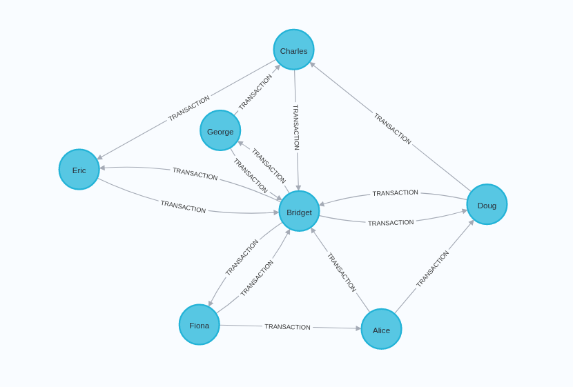
CREATE
  (alice:Person {name: 'Alice'}),
  (bridget:Person {name: 'Bridget'}),
  (charles:Person {name: 'Charles'}),
  (doug:Person {name: 'Doug'}),
  (eric:Person {name: 'Eric'}),
  (fiona:Person {name: 'Fiona'}),
  (george:Person {name: 'George'}),
  (alice)-[:TRANSACTION {value: 81.0}]->(bridget),
  (alice)-[:TRANSACTION {value: 7.0}]->(doug),
  (bridget)-[:TRANSACTION {value: 1.0}]->(doug),
  (bridget)-[:TRANSACTION {value: 1.0}]->(eric),
  (bridget)-[:TRANSACTION {value: 1.0}]->(fiona),
  (bridget)-[:TRANSACTION {value: 1.0}]->(george),
  (charles)-[:TRANSACTION {value: 45.0}]->(bridget),
  (charles)-[:TRANSACTION {value: 3.0}]->(eric),
  (doug)-[:TRANSACTION {value: 3.0}]->(charles),
  (doug)-[:TRANSACTION {value: 1.0}]->(bridget),
  (eric)-[:TRANSACTION {value: 1.0}]->(bridget),
  (fiona)-[:TRANSACTION {value: 3.0}]->(alice),
  (fiona)-[:TRANSACTION {value: 1.0}]->(bridget),
  (george)-[:TRANSACTION {value: 1.0}]->(bridget),
  (george)-[:TRANSACTION {value: 4.0}]->(charles)
With the graph in Neo4j we can now project it into the graph catalog to prepare it for algorithm execution.
We do this using a Cypher projection targeting the Person nodes and the TRANSACTION relationships.
MATCH (source:Person)-[r:TRANSACTION]->(target:Person)
RETURN gds.graph.project(
  'myGraph',
  source,
  target,
  { relationshipProperties: r { .value } }
)
Memory Estimation
First off, we will estimate the cost of running the algorithm using the estimate procedure.
This can be done with any execution mode.
We will use the mutate mode in this example.
Estimating the algorithm is useful to understand the memory impact that running the algorithm on your graph will have.
When you later actually run the algorithm in one of the execution modes the system will perform an estimation.
If the estimation shows that there is a very high probability of the execution going over its memory limitations, the execution is prohibited.
To read more about this, see Automatic estimation and execution blocking.
For more details on estimate in general, see Memory Estimation.
CALL gds.maxkcut.mutate.estimate('myGraph', {mutateProperty: 'community'})
YIELD nodeCount, relationshipCount, bytesMin, bytesMax, requiredMemory| nodeCount | relationshipCount | bytesMin | bytesMax | requiredMemory |
|---|---|---|---|---|
7 |
15 |
488 |
488 |
"488 Bytes" |
Mutate
The mutate execution mode extends the stats mode with an important side effect: updating the named graph with a new node property containing the approximate maximum k-cut for that node.
The name of the new property is specified using the mandatory configuration parameter mutateProperty.
The result is a single summary row, similar to stats, but with some additional metrics.
The mutate mode is especially useful when multiple algorithms are used in conjunction.
For more details on the mutate mode in general, see Mutate.
mutate mode:CALL gds.maxkcut.mutate('myGraph', {mutateProperty: 'community'})
YIELD cutCost, nodePropertiesWritten| cutCost | nodePropertiesWritten |
|---|---|
13.0 |
7 |
We can see that when relationship weight is not taken into account we derive a cut into two (since we didn’t override the default k = 2) communities of cost 13.0.
The total cost is represented by the cutCost column here.
This is the value we want to be as high as possible.
Additionally, the graph 'myGraph' now has a node property community which stores the community to which each node belongs.
To inspect which community each node belongs to we can stream node properties.
CALL gds.graph.nodeProperty.stream('myGraph', 'community')
YIELD nodeId, propertyValue
RETURN gds.util.asNode(nodeId).name as name, propertyValue AS community| name | community |
|---|---|
"Alice" |
0 |
"Bridget" |
0 |
"Charles" |
0 |
"Doug" |
1 |
"Eric" |
1 |
"Fiona" |
1 |
"George" |
1 |
Looking at our graph topology we can see that there are no relationships between the nodes of community 1, and two relationships between the nodes of community 0, namely Alice → Bridget and Charles → Bridget.
However, since there are a total of eight relationships between Bridget and nodes of community 1, and our graph is unweighted assigning Bridget to community 1 would not yield a cut of a higher total weight.
Thus, since the number of relationships connecting nodes of different communities greatly outnumber the number of relationships connecting nodes of the same community it seems like a good solution.
In fact, this is the maximum 2-cut for this graph.
|
Because of the inherent randomness in the Approximate Maximum k-Cut algorithm (unless having |
Mutate with relationship weights
In this example we will have a look at how adding relationship weight can affect our solution.
mutate mode, diving our nodes into two communities once again:CALL gds.maxkcut.mutate(
'myGraph',
{
relationshipWeightProperty: 'value',
mutateProperty: 'weightedCommunity'
}
)
YIELD cutCost, nodePropertiesWritten| cutCost | nodePropertiesWritten |
|---|---|
146.0 |
7 |
Since the value properties on our TRANSACTION relationships were all at least 1.0 and several of a larger value it’s not surprising that we obtain a cut with a larger cost in the weighted case.
Let us now stream node properties to once again inspect the node community distribution.
CALL gds.graph.nodeProperty.stream('myGraph', 'weightedCommunity')
YIELD nodeId, propertyValue
RETURN gds.util.asNode(nodeId).name as name, propertyValue AS weightedCommunity| name | weightedCommunity |
|---|---|
"Alice" |
0 |
"Bridget" |
1 |
"Charles" |
0 |
"Doug" |
1 |
"Eric" |
1 |
"Fiona" |
1 |
"George" |
1 |
Comparing this result with that of unweighted case we can see that Bridget has moved to another community but the output is otherwise the same.
Indeed, this makes sense by looking at our graph.
Bridget is connected to nodes of community 1 by eight relationships, but these relationships all have weight 1.0.
And although Bridget is only connected to two community 0 nodes, these relationships are of weight 81.0 and 45.0.
Moving Bridget back to community 0 would lower the total cut cost of 81.0 + 45.0 - 8 * 1.0 = 118.0.
Hence, it does make sense that Bridget is now in community 1.
In fact, this is the maximum 2-cut in the weighted case.
|
Because of the inherent randomness in the Approximate Maximum k-Cut algorithm (unless having |
Stream
In the stream execution mode, the algorithm returns the approximate maximum k-cut for each node.
This allows us to inspect the results directly or post-process them in Cypher without any side effects.
For more details on the stream mode in general, see Stream.
stream mode using default configuration parameters:CALL gds.maxkcut.stream('myGraph')
YIELD nodeId, communityId
RETURN gds.util.asNode(nodeId).name AS name, communityId| name | communityId |
|---|---|
"Alice" |
0 |
"Bridget" |
0 |
"Charles" |
0 |
"Doug" |
1 |
"Eric" |
1 |
"Fiona" |
1 |
"George" |
1 |
We can see that the result is what we expect, namely the same as in the mutate unweighted example.
|
Because of the inherent randomness in the Approximate Maximum k-Cut algorithm (unless having |