End-to-end workflow
A realistic end-to-end workflow typically involves the use of multiple algorithms in a sequence. This example shows how to create a simple product recommendation engine based on collaborative filtering with the following steps:
-
Create a graph of products and customers.
-
Compute and add node embeddings to the graph with the FastRP algorithm.
-
Compute the similarity score for each pair of customers with the k-Nearest Neighbors (kNN) algorithm based on the node embeddings.
-
Find similar customers and recommend products using Cypher queries.
Create the graph
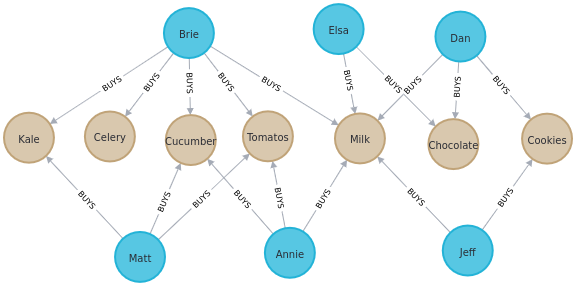
The following Cypher query creates an example graph of products and customers in the Neo4j database.
The amount relationship property represents the average weekly amount of money spent by a customer on a given product.
CREATE
  (dan:Person {name: 'Dan'}),
  (annie:Person {name: 'Annie'}),
  (matt:Person {name: 'Matt'}),
  (jeff:Person {name: 'Jeff'}),
  (brie:Person {name: 'Brie'}),
  (elsa:Person {name: 'Elsa'}),

  (cookies:Product {name: 'Cookies'}),
  (tomatoes:Product {name: 'Tomatoes'}),
  (cucumber:Product {name: 'Cucumber'}),
  (celery:Product {name: 'Celery'}),
  (kale:Product {name: 'Kale'}),
  (milk:Product {name: 'Milk'}),
  (chocolate:Product {name: 'Chocolate'}),

  (dan)-[:BUYS {amount: 1.2}]->(cookies),
  (dan)-[:BUYS {amount: 3.2}]->(milk),
  (dan)-[:BUYS {amount: 2.2}]->(chocolate),

  (annie)-[:BUYS {amount: 1.2}]->(cucumber),
  (annie)-[:BUYS {amount: 3.2}]->(milk),
  (annie)-[:BUYS {amount: 3.2}]->(tomatoes),

  (matt)-[:BUYS {amount: 3}]->(tomatoes),
  (matt)-[:BUYS {amount: 2}]->(kale),
  (matt)-[:BUYS {amount: 1}]->(cucumber),

  (jeff)-[:BUYS {amount: 3}]->(cookies),
  (jeff)-[:BUYS {amount: 2}]->(milk),

  (brie)-[:BUYS {amount: 1}]->(tomatoes),
  (brie)-[:BUYS {amount: 2}]->(milk),
  (brie)-[:BUYS {amount: 2}]->(kale),
  (brie)-[:BUYS {amount: 3}]->(cucumber),
  (brie)-[:BUYS {amount: 0.3}]->(celery),

  (elsa)-[:BUYS {amount: 3}]->(chocolate),
  (elsa)-[:BUYS {amount: 3}]->(milk)
The graph looks as follows:
The next query creates an in-memory graph called purchases from the Neo4j graph.
The only difference from the original data is that the orientation of the :BUYS relationships is discarded; this is because undirected relationships are the default choice when using the FastRP algorithm.
MATCH (source:Person)-[r:BUYS]->(target:Product)
RETURN gds.graph.project(
  'purchases',
  source,
  target,
  {
    sourceNodeLabels: labels(source),
    targetNodeLabels: labels(target),
    relationshipType: 'BUYS',
    relationshipProperties: r { .amount }
  },
  { undirectedRelationshipTypes: ['BUYS'] }
)
Add embeddings to the graph
Node embeddings are commonly used to capture topological information from the graph for further processing, for example to be used by another algorithm.
GDS offers several algorithms to compute embeddings, and FastRP is a good default choice to start with.
Since the embeddings must be available to the kNN algorithm later on, the algorithm must run in mutate mode to add them to the purchases graph.
CALL gds.fastRP.mutate(  (1)
  'purchases',  (2)
  {  (3)
    embeddingDimension: 4,
    iterationWeights: [0.8, 1, 1, 1],
    relationshipWeightProperty: 'amount',
    randomSeed: 42,
    mutateProperty: 'embedding'
  }
)
YIELD nodePropertiesWritten| 1 | gds.fastRP algorithm running in mutate mode. |
| 2 | Name of the projected graph to run the algorithm on and add the new node property to. |
| 3 | Configuration parameters listed in the Syntax section of the algorithm (Mutate mode panel).
Here, the embeddingDimension is set to 4 because the graph is small, the iterationWeights are chosen empirically to yield sensible results, and the relationshipWeightProperty is set to compute weighted averages of the neighboring embeddings.
The randomSeed is added to obtain the same results for every run, but is not necessary for the actual computation.
The mutateProperty is the new node property that will contain the node embedding. |
| nodePropertiesWritten |
|---|
13 |
You can run the algorithm in stream mode as in the Basic workflow example by using the corresponding gds.fastRP.stream procedure and removing the mutateProperty from the configuration parameters.
Compute and write similarities
With the embeddings available as the new embedding node property, you can run the kNN algorithm to compute a similarity score between each pair of nodes.
Run the kNN algorithm in write mode to add the score relationship to the Neo4j database and use it in Cypher queries.
CALL gds.knn.write(  (1)
  'purchases',  (2)
  {  (3)
    nodeProperties: ['embedding'],
    nodeLabels: ['Person'],
    topK: 2,
    sampleRate: 1.0,
    deltaThreshold: 0.0,
    randomSeed: 42,
    concurrency: 1,
    writeProperty: 'score',
    writeRelationshipType: 'SIMILAR'
  }
)
YIELD similarityDistribution
RETURN similarityDistribution.mean AS meanSimilarity (4)| 1 | gds.knn algorithm running in write mode. |
| 2 | Name of the projected graph to run the algorithm on.
The write mode does not update the in-memory graph. |
| 3 | Configuration parameters listed in the Syntax section of the algorithm (Write mode panel).
The nodeLabels option is set to ['Person'], because we are interested only in Person-Person similarities and don’t want to mix up such similarities with e.g. Person-Product similarities.
Here, topK is set to 2 to select only the two closest targets of a source node, while the sampleRate and the deltaThreshold are set to 1 and 0 respectively because the graph is small.
The concurrency and the randomSeed are set to obtain the same results for every run, but are not necessary for the actual computation.
The two write properties are used to write a new :SIMILAR relationship with a score property containing the similarity score between two nodes. |
| 4 | mean is one of the fields of the returned similarityDistribution map. |
| meanSimilarity |
|---|
0.8800284068 |
The mean similarity between nodes is high.
This is because the similarity distribution is computed after selecting the topK=2 most similar targets per source node. Moreover, the graph has two clusters of users with quite similar purchases: (Brie, Matt and Annie) and (Elsa, Dan and Jeff). Using a higher value for topK would yield a lower average similarity.
If we were to examine Person-Product similariteies, this could be accomplished by using instead Filtered K-Nearest Neighbors.
Find the most similar nodes
After writing the similarity relationships to Neo4j, you can use Cypher to find pairs of customers and rank them by their similarity score.
MATCH (n:Person)-[r:SIMILAR]->(m:Person)
RETURN n.name AS person1, m.name AS person2, r.score AS similarity
ORDER BY similarity DESCENDING, person1, person2| person1 | person2 | similarity |
|---|---|---|
"Dan" |
"Elsa" |
0.9866833091 |
"Elsa" |
"Dan" |
0.9866833091 |
"Brie" |
"Matt" |
0.9740184546 |
"Matt" |
"Brie" |
0.9740184546 |
"Annie" |
"Matt" |
0.9724045992 |
"Matt" |
"Annie" |
0.9724045992 |
"Annie" |
"Brie" |
0.9154552221 |
"Brie" |
"Annie" |
0.9154552221 |
"Jeff" |
"Annie" |
0.8667784333 |
"Jeff" |
"Matt" |
0.7591181397 |
"Dan" |
"Jeff" |
0.6660436392 |
"Elsa" |
"Jeff" |
0.5712890029 |
The query result shows that the nodes named "Dan" and "Elsa" are very similar.
In fact, they are both connected to three :Product nodes, two of which are the same (the nodes named "Milk" and "Chocolate") and with similar amounts. The "Cookies" Product is only purchased by Dan, but with a lower amount, and it also has a certain degree of similarity to the other products due to its proximity in the graph and partly due to randomness.
Make recommendations
The basic assumption of collaborative filtering is that products purchased by a customer may be of interest for a similar customer who is not already buying them. Knowing that "Annie" and "Matt" are similar, you can make product recommendations for each of them with a Cypher query.
MATCH (:Person {name: "Annie"})-->(p1:Product)
WITH collect(p1) AS products
MATCH (:Person {name: "Matt"})-->(p2:Product)
WHERE NOT p2 IN products
RETURN p2.name AS recommendation| recommendation |
|---|
"Kale" |
The query looks for products that "Annie" is buying, then selects the products that "Matt" is buying which "Annie" is not buying yet. The resulting node "Kale" is therefore the recommended product for "Annie".