Driving Predictive Analytics with the Power of Neo4j

Editor’s Note: This presentation was given by Blake Nelson and Deve Palakkattukudy at GraphConnect San Francisco in October 2016.

Presentation Summary

Agero has been the industry leader in roadside assistance for the last 40 years. Much of their business depends on locations — the location of customers, predictive locations of service providers, tracking locations and roadways — the speed on any given road, and countless other data points. As soon as Agero realized the nature of their connected data, they turned to the power of Neo4j.

The company is using the graph database to create an open source spatial plugin using crowdsourced OpenStreetMap (OSM) data to detect changing roadway and driving conditions, analyze dynamic conditions for developing trends, predict potential consequences of those trends, and improve driver safety and the driving experience.

The OSM data structure is based on hierarchical data that consists of nodes (latitude and longitude locations), ways (a collection of nodes) and relationships. Relying on unique node IDs and the relationships between these nodes, they are able to provide drivers with real-time driving conditions.

So why did the company choose Neo4j? Because of the Bolt protocol, stored procedures and plugin capabilities it provides – which has allowed Agero to easily interface with the graph database using their existing processes and programming languages.

Full Presentation: Driving Predictive Roadway Analytics with the Power of Neo4j

Blake Nelson: What we’re going to be talking about today is how Agero uses Neo4j to create predictive roadway analytics for drivers and their related service companies:



I’m the principal, founder and owner of Waveonics, a small software development firm. I’ve been working with Agero on a project we’ll be going over shortly, and I’m going to talk a little bit about the experience as a small business partnering with an industry powerhouse.

Agero is a leading provider of vehicle and driver safety, security and information services while Waveonics is a software development and consulting firm. Together, we are leveraging Neo4j to create an open source spatial plugin using crowdsourced OpenStreetMap (OSM) data to detect changing roadway and driving conditions, analyze dynamic conditions for developing trends, predict potential consequences of those trends, and improve driver safety and the driving experience.

Driving conditions are dynamic because they’re affected by factors such as weather, traffic and construction. We now have the ability to gather and analyze data from our customers to start employing better predictive analytics and machine learning. This allows us to make predictions and adjustments to increase the safety of the driving experience.

I was brought in to help analyze different graph database technologies. We’ll go over our use case, our experience with Neo4j, some of the issues we’ve encountered and the flexibility of the environment.

Agero: Industry Leader in Roadside Assistance

Deve Palakkattukudy: Agero has been in the roadside assistance business for the last 40 years:



We help subscribers if their car breaks down, if their car needs a repair or if a driver gets in an accident. We connect the auto manufacturers, insurance companies, dealers, financial institutions and towing companies so that we can provide roadside assistance and end-to-end accident management services.

We have been the industry leader in the roadside assistance business for the last 40 years, and we have more than 9.5 million dispatches per year — for both roadside assistance and travel accident management. We service more than 75% of new passenger cars, which is one out of every 20 cars on the road.

We support more than 350 APIs, most of which are publicly available, and have pioneered cutting-edge telematic solutions that are currently being installed in high-end cars. Today our engineering team is working on a next-gen telematics platform with data we collect from cell phone sensors, and we’re currently able to predict accidents.

We rely on data we have collected over the last 40 years, a large amount of which is location-based — the location of our customers, predictive locations of our service providers, tracking locations and roadways — and the speed on any given road. All of this data is connected back to our customer. As soon as we realized the connected nature of our data, we turned to the power of Neo4j in our Agero engine.

Using Open Source Data to Power Predictive Analytics

Nelson: We are working with 85 million drivers and dispatching nearly 10 million calls annually. We can combine this data with the data we are collecting from the sensors in people’s cell phones to detect an accident in nearly real time. We’re also able to understand travel patterns using that same cell phone sensor.

By using these analytics, we can start making predictions and determine how to feed them back to our major clients: insurance companies, service providers and financial companies. And Agero is the glue that holds the driver together with all of the companies that are selling to them.

We’re focused primarily on roadways, travel and navigation — so how do we get the data we need to populate the database? We use crowdsourced data, similarly to the way Waze – a small company purchased by Google — uses data.

This open source, crowdsourced data is put in by a vast number of worldwide users from engineers, GIS professionals, mappers and humanitarians. If you need to get information about how to react to a typhoon or hurricane, where can you find it and how can you effectively deploy assistance?

Our data comes from GIS databases; open source databases such as the government’s census databases; open source data from local sources that includes property ownership, geographic boundaries, roadways, etc.; and existing low-tech maps. All of these sources come together to create OSM, so it’s a rich set of data we have at our disposal. And this is the use case we plan to discuss.

The Hierarchy: OneStreetMap Data Structure

OSM is build upon a hierarchy of information. We start with points, which are our nodes, that are at the lowest level. These consist of latitude and longitude, each of which consists of a globally unique ID along with tags that are key-value properties.

Because these tags come from external sources, they could be literally anything — which can also be a downside. For example, is a highway spelled highway, or H-W-Y? They mean the same thing to us semantically, but it’s a harder to capture that within the data model effectively.

On top of the nodes we have an ordered sequences of nodes in the form of a “way,” or route. These consist of “way” IDs and a sequence of “node” IDs, which may have tags that are key-value properties. They are a coordinated sequence of GPS points that could be anything from a short region of roadway or train tracks to river ways or bike paths. So you can start describing certain areas and regions, the speed limit in those areas, etc.

The very top semantic is the “relation,” which could refer to a set of latitude/longitude node points, an organization sequence of the “ways” that we just discussed, or it could reference a subrelation. This logic starts building polygons — or areas — such as the boundaries of a town, city, lake or an office park. This provides rich semantic information, and we build this up level by level within OpenStreetMap.

Putting the Data to the Test

Below is what this looks like in XML:



We have the unique node ID, a latitude/longitude position, and then possibly a tag, key-value pair or organization. Here we’ve got a GPS that represents the position of a traffic sign, and then on top of that we have “ways” with a reference — which they call ND for clarity (node references) — that point back to a previous node ID in the file. Following that, we have the relationships down at the bottom, where we refer back to any preceding relationship way or node:



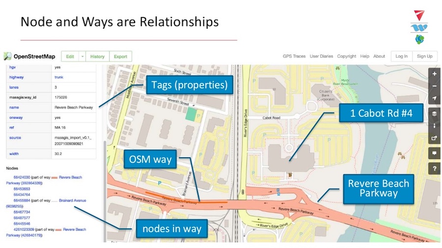
1 Cabot Road #4 is the office location for Agero, just outside of Boston. The area highlighted in orange at the bottom is Revere Beach Parkway and represents only a section of the road. Listed at the very bottom we have a number of nodes that exist in the “way,” and all of these unique IDs can be part of multiple ways.

Our data also tells us we have an intersection between Revere Beach Parkway and Brainard Avenue. Our key-value pairs, which happen to be a reference, came from the MassGIS database and shows that the width of the road is 30.2 meters wide.

This has a fair amount of scale and complexity to it. The ways can be roads, trails, bike paths, waterways, rivers, train tracks – anything that’s of interest to somebody who’s mapping.

The data is also incredibly dynamic. For example, a snapshot from a couple of weeks ago shows that for a given day there were 1.2 million additions, 302,000 modifications and 120,000 deletions. In North America alone we have close to one billion nodes of latitude/longitude points, over 60 million “ways” (sequence of related nodes), 330 million tags (properties of nodes and ways), and 972,000 “relations” (between ways and nodes). The number of users and contributors has also been increasing steadily.

Each “way” is unique:



They each have some combination of information — such as the surface conditions of a road and its speed limit — so that we can understand what our drivers face and how to best serve them.

Even in areas where we don’t have information in the database, we can analyze the data we have on the surface condition, the time of the day and the weather to make intelligent predictions about what the effective speed should be. If we see outliers from that, we may be working with an unsafe driver.

If you look at our orange roadway, we have about a half dozen different OSM ways that are connected because one meter of road can vary from the next meter of road.

Choosing Neo4j

So why did we decide to make the transition to a graph database? Because roadways are graphs:



We start somewhere, we go somewhere, we follow the roadway and we turn it into sections. As we understand the location information coming from our users as they drive their cars, we can pick up the sensor and GPS information.

We need to map this back to where the actual roads are so that we can understand the driver’s behavior and the properties of the road. How will they drive in that location? Is it safe? Should we reroute them if we’re dealing with the fleet, or travel, or service providers?

Each of these segments — which are edges between the nodes — has properties we want to represent. Neo4j gives us the capability to put properties on these edges and the relations between their nodes. That’s a lot easier to do in the graph database model than in our relational database model.

Bolt Protocol

As we saw the capabilities that were being delivered in Neo4j, we saw how useful the graph database could be for us. The first comes in the form of Neo4j’s Bolt protocol, which currently includes native drivers for Python, Java, Javascript and .NET.

Our data scientists work with machine learning programs that include standard algorithms, much of which are done in Python. A lot of our developers also work in Java and we have multiple platforms run in JavaScript for our web pages. But we have support for all of these through the native Neo4j Bolt protocol.

The ability to bring in a tool like Neo4j that fits easily with the way we develop is a huge plus for us. We can also use it to richly model our data because it fits our use case, and it allows us to access our data in a way we already operate.

Stored Procedures

Stored procedures are another big win for us. Much of our work is investigative in nature, because we are always seeking to learn more from the data coming in.

Our data scientists are creating algorithms, and if we want to ramp up performance, we can move these algorithms into stored procedures. We can move the processing closer to the data, and get the power out of the server rather than on the client. So we develop our client, and we migrate over to the server as our performance teams provide.

Plugin Capabilities: Rtree and GeoHash

Neo4j also has a plugin tech capability. I work with the Neo4j Spatial plugin, which has native support to import OpenStreetMap data and builds an Rtree-based index.

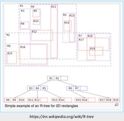
RTree is a way to balance geolocations. Given latitudes and longitude, you figure out the bounding box for the entity of interest and break the world into rectangles, balancing out the allocation of the entries into those rectangles:



You have minimization of bounding boxes, and then you build a tree with children. As you walk down the tree for any of these bounding boxes, if you find your point of interest you start searching the children to see if you can have a smaller, more refined bounding box.

Unfortunately, Rtrees don’t perform well at scale, particularly in worst-case scenarios. If the data you bring in continually changes, you can end up with overlaps in the bounding boxes. Sometimes you need to split and rebalance the tree, which takes a lot of reprocessing.

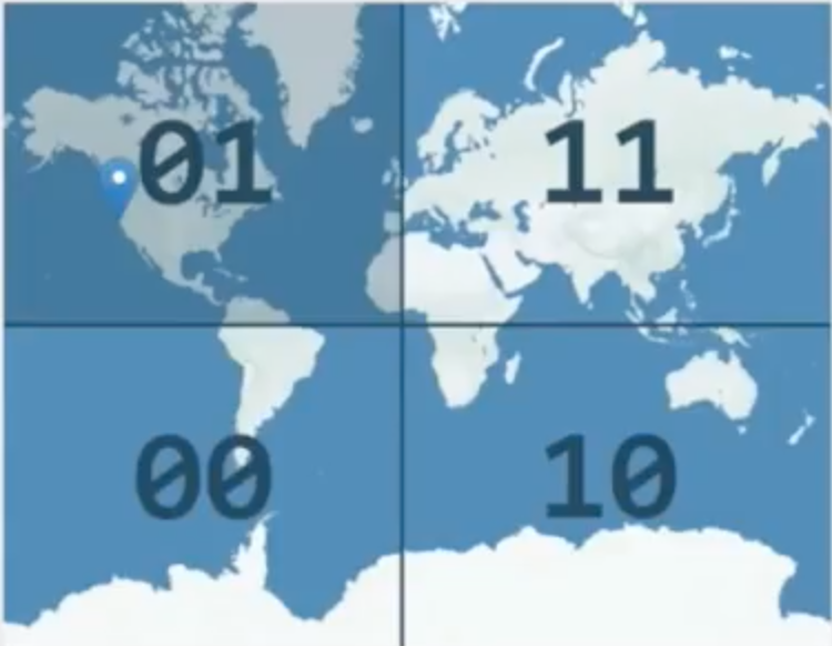
Another way you can index is with GeoHash, which allows you to take a two-dimensional latitude, longitude and break it into a one-dimensional bit string. We take the world, and we split it into “cells” — first via longitude to determine which side of the world you’re on, the left or the right. If you’re on the right, you get a 1, and if you’re on the left you get a 0:



Next you split by latitude. If you’re north, you get a 1 and If you’re south, you get a 0:



We can keep splitting until we get down to whatever level of granularity we want to work with.

As we split things out, things that are close to one another will be in the same bounding box and will therefore have the same preceding bit string, so you can end up with something like this:



You take the latitude and longitude, continue splitting the world in half and end up with a bit string. If we take our location here at (37.7, -122.41), it puts us right at GraphConnect.

When we split it a whole bunch of times we end up with a long, unmanageable bit string. But if you take that and you build in characters with five bits at a time – base 32 encode it – you get something that’s more readable.

So we go from latitude and longitude to our bit string at base 32 encoded, and we come up with 9q8yy for our region with some amount of variant. Depending on how long the string is, you get a smaller bounding box. With a shorter string, you get a larger bounding box. All we’re doing is dividing and bit shifting, so it’s nice, quick encoding that takes us from two-dimensional to one-dimensional.

And we can reverse it almost as quickly:



We can go from one-dimension to two-dimension by following the same steps in reverse. Take our base 32, put it to our bit string, and then — knowing that every other bit has meaning for either latitude or longitude — we can calculate by pulling out the bits and rebuilding our latitude and longitude.

But it’s important to remember that these coordinates are not the actual point — they represent a bounding box, so there’s some amount of error in there. The longer the string, the less the error, so it’s a trade-off.

We can also use this data to determine closeness:



Almost everything that’s right around us is going to be in this bounding box, or in one of the surrounding bounding boxes — which means a different string. It’s going to be in one of those nine areas, and we make the bounding boxes smaller by making the string a little longer or vice versa. This is an incredibly flexible encoding mechanism.

We can look up that string really quickly using graph technology. If we build a GeoHash tree using our string, we can put identifications on each of the relationships between the node in our tree. We follow the string down the graph and end up at the leaf that represents San Francisco:



To find locations that are close to us, we’re either going to come down to the same node, or we’re going to have a GeoHash of one of the neighbors and follow quickly down that path, until we get towards the end and then we branch off.

This is what it looks like when we put it into Neo4j:



For these five GeoHash strings, I have the same predecessors for the character string, and then eventually, on the last code, I’m either a Y or a W, and I branch out. We have a unique character for the last of the string and then we get our leaf nodes. Next I take each of my leaf nodes to form a relationship to the OSM way of interest.

As I pull in the information from OpenStreetMap and I look at each of the ways, I can determine which GeoHash regions that way is going to intersect with, and then associate that way with the GeoHash string in my tree.

So when I’m out looking for a driver based on a positional reading (latitude, longitude) I can use GeoHash to determine where the driver is, encode that GeoHash, walk my tree and get to a leaf node that is going to point me to the set of OpenStreetMap ways closest to me. I can do that for the balance of the neighbors as well.

This gives me a quick way to look at where the driver is based on GPS readings. Within some error-reading from the GPS through buildings or chips in his mobile device, I can figure out what’s within that closeness based on how large I’ve made my GeoHash regions. I’m able to tie in my indexing of the region with the actual data in the same graph without any real confusion of what I’m processing.

Why the Neo4j Graph Database?

Because I have Neo4j that’s an open source capability, and because I have the ability to go in and build my own stored procedures or modify the existing stored procedures that are in there for the Neo4j Spatial plugin, I can enhance the existing Rtree — which doesn’t perform the way I need it to — and enhance it with a different way to index and look up my information.

Our environment is rich enough to represent the complexity and relationships from OpenStreetMap between my corporate customers, service providers and the 85 million people on the road who are tied in with my technology — and glue all of those together via known data relationships.

I can run analytics on the data from those relationships and use them because the data is tuned for my use case. And while I didn’t like the performance of the Rtree based on my particular use case, I can easily modify it.

We can take our directed graph along with the Neo4j Spatial plugin that’s natively supporting the OpenStreetMap data and customize it for the datasets we’ve uploaded. I can modify the indexing to fit my use case, and I can depend on the performance of Bolt to give my data scientists the flexibility to continue working with the tools they have.

The Agero developers with Java backgrounds can easily move into this environment. I can optimize my performance by taking skunk work algorithms and — as they formalize and validate — can move them into stored procedures and bind them to the database.

I have open source code and the community support from Google Groups and OpenStack that I can go to for support, and I can build up my own functionality with the plugin capability. I can tune this when we put in our own algorithms and our proprietary information that allows us to connect our corporate and our driving customers that we’re working with. All of this flexibility of the environment is extremely helpful for us.