Graph Algorithms in Neo4j: Closeness Centrality


5 min read
Graph algorithms provide the means to understand, model and predict complicated
dynamics such as the flow of resources or information, the pathways through which
contagions or network failures spread, and the influences on and resiliency of groups.
This blog series is designed to help you better utilize graph analytics and graph algorithms so you can effectively innovate and develop intelligent solutions faster using a graph database like Neo4j.
Last week we continued our look at Centrality algorithms, with a focus on Betweenness Centrality, which measures the number of shortest paths that pass through a node.

This week we’ll move further into Centrality algorithms, with a focus on Closeness Centrality, which measures how central a node is within its cluster. Nodes with the shortest paths to all other nodes are assumed to
be able to reach the entire group the fastest.
About Closeness Centrality
Closeness Centrality is a way of detecting nodes that are able to spread information efficiently through a graph.
The Closeness Centrality of a node measures its average farness (inverse distance) to all other nodes. Nodes with a high closeness score have the shortest distances to all other nodes.
For each node, the Closeness Centrality algorithm calculates the sum of its distances to all other nodes, based on calculating the shortest paths between all pairs of nodes. The resulting sum is then inverted to determine the Closeness Centrality score for that node.
NOTE: The raw Closeness Centrality of a node is calculated using the formula:
raw closeness centrality(node) = 1 / sum(distance from node to all other nodes)It is more common to normalize this score so that it represents the average length of the shortest paths rather than their sum. This adjustment allows comparisons of the Closeness Centrality of nodes of graphs of different sizes.
The formula for normalized Closeness Centrality is as follows:
normalized closeness centrality(node) = (number of nodes - 1) / sum(distance from node to all other node
When Should I Use Closeness Centrality?
- Closeness Centrality is used to research organizational networks where individuals with high Closeness Centrality are in a favorable position to control and acquire vital information and resources within the organization. One such study is “Mapping Networks of Terrorist Cells” by Valdis E. Krebs.
- Closeness Centrality is also interpreted as an estimated time of arrival through telecommunications or package delivery networks where content flows through shortest paths to a predefined target. It is also used in networks where information spreads through all shortest paths simultaneously, such as infections spreading through a local community. Find more details in “Centrality and Network Flow” by Stephen P. Borgatti.
- Closeness Centrality helps estimate the importance of words in a document, based on a graph-based keyphrase extraction process. This process is described by Florian Boudin in “A Comparison of Centrality Measures for Graph-Based Keyphrase Extraction.”
NOTE:
Academically, Closeness Centrality works best on connected graphs. If we use the original formula on an unconnected graph, we end up with an infinite distance between two nodes in separate connected components. This means that we’ll end up with an infinite Closeness Centrality score when we sum up all the distances from that node. In practice, a variation on the original formula is used so that we don’t run into these issues.
Closeness Centrality Example
Let’s see how Closeness Centrality works on a small dataset.
The following Cypher statement creates a graph with nodes and links between them:
MERGE (a:Node{id:"A"})
MERGE (b:Node{id:"B"})
MERGE (c:Node{id:"C"})
MERGE (d:Node{id:"D"})
MERGE (e:Node{id:"E"})
MERGE (a)-[:LINK]->(b)
MERGE (b)-[:LINK]->(a)
MERGE (b)-[:LINK]->(c)
MERGE (c)-[:LINK]->(b)
MERGE (c)-[:LINK]->(d)
MERGE (d)-[:LINK]->(c)
MERGE (d)-[:LINK]->(e)
MERGE (e)-[:LINK]->(d);

The following query executes the Closeness Centrality algorithm:
CALL algo.closeness.stream("Node", "LINK")
YIELD nodeId, centrality
MATCH (n:Node) WHERE id(n) = nodeId
RETURN n.id AS node, centrality
ORDER BY centrality DESC
LIMIT 20;


C is the best connected node in this graph, although B and D aren’t far behind. A and E don’t have close ties to many other nodes, so their scores are lower. Any node that has a direct connection to all other nodes would score 1.
Harmonic Centrality
Harmonic Centrality (also known as Valued Centrality) is a variant of Closeness Centrality that was invented to solve the problem the original formula had when dealing with unconnected graphs. As with many of the centrality algorithms, it originates from the field of social network analysis.
Harmonic Centrality was proposed by Marchiori and Latora in “Harmony in the Small World” while trying to come up with a sensible notion of “average shortest path.”
They suggested a different way of calculating the average distance to that used in the Closeness Centrality algorithm. Rather than summing the distances of a node to all other nodes, the Harmonic Centrality algorithm sums the inverse of those distances. This enables it to deal with infinite values.
NOTE:
The raw harmonic centrality for a node is calculated using the following formula:
raw harmonic centrality(node) = sum(1 / distance from node to every other node excluding itself)As with Closeness Centrality we also calculate a normalized harmonic centrality with the following formula:
normalized harmonic centrality(node) = sum(1 / distance from node to every other node excluding itself) / (number of nodes - 1)In this formula, ∞ values are handled cleanly.
Conclusion
As we showed in our look at the Closeness Centrality algorithm, Closeness Centrality is applicable in a number of resource, communication and behavioral analyses, especially when interaction speed is significant.
Next week we’ll begin our exploration of Community Detection Algorithms, with a look at the Strongly Connected Components algorithm.
Learn about the power of graph algorithms in the O’Reilly book,
Graph Algorithms: Practical Examples in Apache Spark and Neo4j by the authors of this article. Click below to get your free ebook copy.
Share Article


Explore
Related Articles

Mastering Fraud Detection With Temporal Graph Modeling

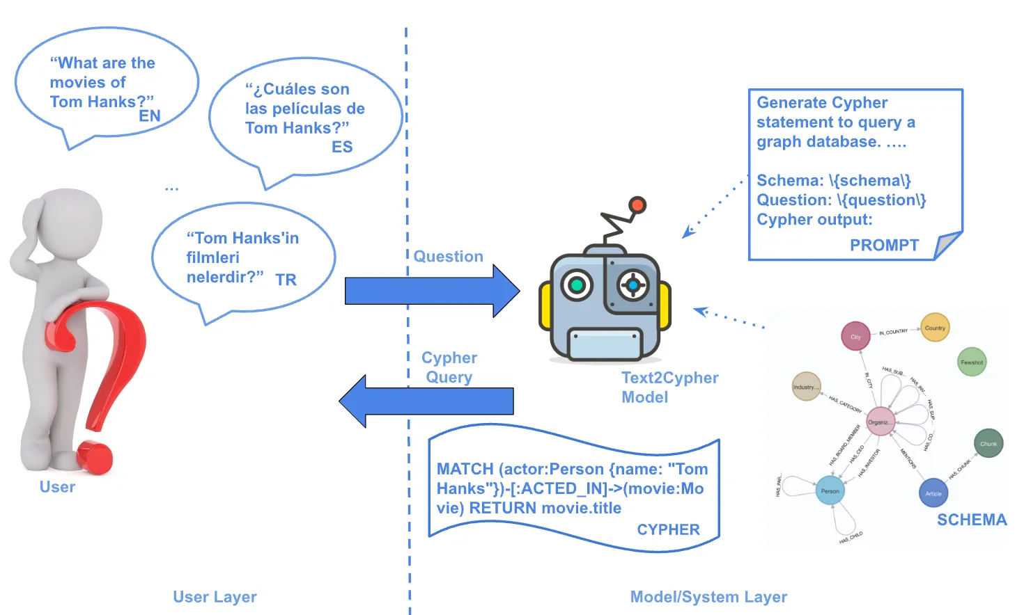
Text2Cypher Across Languages: Evaluating Foundational Models Beyond English