A machine learning innovation in predictive analytics

Senior Field Engineer, Neo4j
16 min read

Some say you get better predictions with graph data science.
The idea looks beautiful and indeed graphs are powerful tools. We would like to prove as hard as marble that connected data render predictions far more accurate. And measure how much more.
Let’s do it on the CORA dataset of scientific publications, well-known in the data science ecosystem: Neo4j and graph embeddings allow you to gain several points of accuracy to predict the category of a given research paper.
Introduction
The blog structure is as follows: first, we introduce the graph technology and the Neo4j graph platform. Then, we dig deeper into the Neo4j Graph Data Science. Finally, we switch to the demo that leverages the Neo4j GDS. You can go straight to that section if you already have a good understanding of the Neo4j ecosystem. At the end, we wrap up the key takeaways of this blog post.
The graph technology
Graph technology unifies data relationships in a more intuitive, connected state, unlocking deeper context.

Fig. 1 – A graph (of people, transactions, etc.) connects data as nodes and relationships
Once data is stored as a graph, you start understanding how it is connected – sometimes a link between two nodes is not visible in other technologies because they are multiple hops away from each other. In short, graph databases allow you to traverse deep paths throughout your connected data. Incredible insights are revealed through graphs.
Neo4j is the category creator and leader in graph databases, the fastest growing category in all of data management. Neo4j has over 300 Global Enterprise customers and 800+ total customers.
The Neo4j graph platform

Fig. 2 – The Neo4j graph platform
Let us briefly describe the Neo4j graph platform, composed of:
- The Neo4j Graph Database is a native graph data store built from the ground up to leverage not only data but also data relationships. Unlike other types of databases, Neo4j connects data as it’s stored, enabling queries never before imagined, at speeds never thought possible.
- Neo4j Graph Data Science is a software platform helping data scientists uncover the connections in big data to answer business critical questions and improve predictions.
- Neo4j Bloom is an easy-to-use graph exploration application for visually interacting with Neo4j graphs. Bloom gives graph novices and experts alike the ability to visually investigate and explore graph data from different business perspectives.
- Cypher Query language: With Neo4j, connections between data are stored – not computed at query time. Cypher is a powerful, graph-optimized query language that understands, and leverages, these stored connections.
- Neo4j offers several connectors to facilitate use of Neo4j in your particular architecture, and provides instructional support for some third-party and community tools. Neo4j connects with Apache Spark and Apache Kafka, as well as with various BI tools and data science studios. Neo4j official drivers support Java, JavaScript, python, .Net, and Go, and GraphQL support is top notch with the GRANDstack baseline architecture.
- Neo4j developer tools are sophisticated tools provided by Neo4j and designed to make it easier to develop graph applications. They include Neo4j Desktop to create graph projects, Neo4j Browser to query your graphs as well as Neo4j Data Importer to quickly load your data into your graph.
The Neo4j Graph Platform can run on a variety of cloud deployment options readily available. Over 50 percent of Neo4j customers run Neo4j in the cloud today on public clouds like AWS, Azure, and Google Cloud Platform (GCP). Of course, Neo4j also runs on-prem, in private clouds or in hybrid environments.
We will now zoom in on Neo4j Graph Data Science.
Neo4j graph data science
“Data can’t save you if you don’t have a question…” Who said that? I can’t remember.
Anyway, what sort of data questions does Neo4j Graph Data Science allow me to answer?
They could be summarized as a three-stage progression:
- What’s important?
- What’s unusual?
- What’s next?
For each of these questions, the Neo4j graph database provides an efficient answer:
- To identify what’s important in your data, you first need to connect entities together with relationships and build a knowledge graph. Then you’re able to find the patterns you’re looking for in your connected data (using Cypher queries and graph patterns).
- To detect outliers, clusters, and trends, there are 65+ graph algorithms available in the Neo4j Graph Data Science library.
- To predict the future, we feed machine learning models with graph features and improve prediction accuracy. The Neo4j Graph Data Science library includes three different pipelines: node classification, node regression, and link prediction

Fig. 3 – Climb to the next Graph Data Science Maturity Level!
In a sense, you can consider these three steps as your graph data science maturity level. The more you grow your use cases trying to solve the three questions, the higher you climb in the graph data science maturity ladder.
Why use Neo4j Graph Data Science?
Benefits:
There are four key advantages of the Neo4j Graph Data Science:
- Easy to use: low-code and no-code tools, integrations, workflows. Also – quick on-boarding via cloud, tight integration, and automation of workflow elements.
- Data Scientists: widest breadth of data science algorithms, language support – like Python, easy connectivity to both data sources, and ML tools.
- Enterprise Ready: performance, reliability, and architectural integrity to meet customer needs at any scale.
- Ecosystem: providing easy interconnecting to both data systems (Lakes, Warehouses, etc..) and other technologies like GCP Vertex AI, AWS SageMaker, and Azure Synapse.

Fig. 4 – Benefits of using the Neo4j Graph Data Science
Algorithms and machine learning
The algorithms available in the Neo4j Graph Data Science library fall into six main categories:
Supervised ML includes pipelines for node regression, node classification, and link prediction.
There are also many useful auxiliary functions and procedures. Last but not least, the Pregel Java API enables you to build your own algorithms by implementing several interfaces.

Fig. 5 – Over 65 Pretuned, parallelized algorithms
From chaos to structure
Neo4j Graph Data Science is literally changing how machine learning gets done.

Fig. 6 – Node embeddings capture any node into a vector
Graph Embeddings summarize the enhanced explicit knowledge of a graph while ensuring dimensionality reduction. The embedding vector – because it absorbs the network topology – turns out to be a highly predictive feature when added to a given machine learning pipeline.
Let us now succinctly describe the CORA dataset before moving to the hands-on, practical part.
The CORA dataset

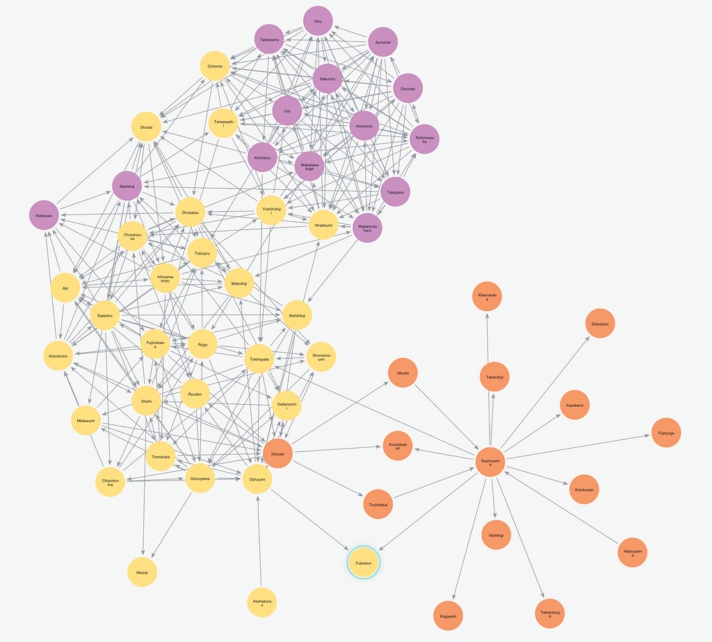
Fig. 7 – CORA citation graph (Source: https://paperswithcode.com/dataset/cora)
The CORA dataset is called “the MNIST of graph land.” It is composed of 2708 academic papers (Paper nodes), categorized into seven classes (“Theory,” “Reinforcement learning,” “Probabilistic methods, etc.)
There are 5429 edges connecting the research papers (CITES relationships).
Regarding properties, there is a 1433 feature vector per node extracted from the paper text.
Let’s play the notebook
Just open the Python notebook from github and follow the commands. You can import it in your Google Drive from github or simply clone the github project. I’ll try my best to answer comments and manage pull requests.
The whole data processing and machine learning can be run from the sole notebook. You will only need:
- a running Neo4j instance with the graph data science plugin
AND
Spawn your Aura DS instance
This is the first step. The magic won’t happen without a Neo4j instance. We suggest to use Neo4j AuraDS to spawn a self-managed Neo4j instance, equipped with the Neo4j Graph Data Science plugin. You could as well use a Neo4j Sandbox for graph data science.
Once you are down, you can pause or stop your instance.

Fig. 8 – Select your DS instance on the Neo4j Aura console
Once you have spawned your instance, you are prompted to download a .env file that contains your credentials to connect to the Neo4j AuraDS instance.
Please upload that .env file to the G Drive root folder associated to the Colab notebook.

Fig. 9 – Upload your .env file containing AuraDS credentials
Install Graph Data Science Python client
The Neo4j graph data science python client is installed on your notebook via a !pip install command.

Fig. 10 – Install graphdatascience python client
Secure our database credentials
Next step is to secure our credentials to connect to the Neo4j database.
You will need to install the python-dotenv package.
!pip install python-dotenv
Then, execute this code:
from dotenv import load_dotenv
import os

load_dotenv("/content/credentials-xxxxxx.env")

bolt = os.getenv("NEO4J_URI")
user = os.getenv("NEO4J_USERNAME")
password = os.getenv("NEO4J_PASSWORD")
In the remainder of the notebook, we can now manipulate these variables without displaying them explicitly.
Instantiate Graph Data Science Python client
Let’s now obtain a new graphdatascience client:
import pandas as pd
from IPython.display import display

from graphdatascience import GraphDataScience

gds = GraphDataScience(bolt, auth=auth, aura_ds=True)
We can display the gds client version:
print(gds.version())

2.1.9
Load the CORA dataset
It’s time to load the CORA dataset into the Neo4j graph database. Two Cypher commands will be used for ingestion, 1 for Paper nodes and 1 for CITES relationships. Those Cypher commands will be run through the run_cypher method of the python client.
node_load_q = """LOAD CSV WITH HEADERS FROM "https://raw.githubusercontent.com/Kristof-Neys/Neo4j-Cora/main/node_list.csv" AS row
WITH toInteger(row.id) AS paperId, row.subject AS subject, row.features AS features
MERGE (p:Paper {paper_Id: paperId})
SET p.subject = subject, p.features = apoc.convert.fromJsonList(features)
RETURN count(p)
"""


edge_load_q = """
LOAD CSV WITH HEADERS FROM "https://raw.githubusercontent.com/Kristof-Neys/Neo4j-Cora/main/edge_list.csv" AS row
MATCH(source: Paper {paper_Id: toInteger(row.source)})
MATCH(target: Paper {paper_Id: toInteger(row.target)})
MERGE (source)-[r:CITES]->(target)
"""
gds.run_cypher(node_load_q)
gds.run_cypher(edge_load_q)
Alright, let’s visualize right now the CORA graph in Bloom: (please access Bloom from your AuraDS console or from the sandbox)

Fig. 11 – Visualize the CORA graph in Neo4j Bloom
Quick peek at the features
The features describing each paper in the CORA dataset were stored as a node property on each Paper node.
q_peak = """MATCH (n) WHERE EXISTS(n.features) RETURN DISTINCT n.paper_Id as PaperId, n.subject  AS Paper_Subject, n.features AS features LIMIT 5"""
res = gds.run_cypher(q_peak)
df = pd.DataFrame.from_dict(res)
display(df.head(5))

Fig. 12 – CORA Paper ids, subjects and features
The features property is an array (a vector) of size 1433 containing 0 and 1 values.
Paper subject is a string property. We want to refactor it into an Integer:
query_Subj = """MATCH (p:Paper)
WITH collect(DISTINCT p.subject) as listSubjects
WITH  listSubjects, size(listSubjects) AS sizeListSubjects
WITH listSubjects, range(1, sizeListSubjects) AS rangeSubjects
WITH apoc.map.fromLists(listSubjects, rangeSubjects) AS mapSubjects
MATCH (p:Paper)
SET p.subjectClass = mapSubjects[p.subject];"""

gds.run_cypher(query_Subj)
Time to start the GDS engines
We’d like to project the CORA graph into memory so as to compute embeddings based on the Paper nodes and the CITES relationship.
G, res = gds.graph.project(
   "cora-graph",
   {"Paper": {"properties": ["subjectClass", "features"]} },
   {"CITES": {"orientation": "UNDIRECTED", "aggregation": "SINGLE"}}
)
Let’s learn some information about the in-memory graph:
print(G.name())             # cora-graph
print(G.memory_usage())     # 30 MiB
print(G.density())          # 0.0014399999126942077
FastRP time!
We will use the FastRP algorithm (FastRP stands for Fast Random Projection) to compute node embeddings for each Paper node. This algorithm enables each node to be projected into a vector of reduced dimension, while preserving pairwise distances between the nodes.
A small explanation here:
- we have 2708 Paper nodes
- we will compute an embedding for each of them
- the embedding dimension will be reduced from 2708 to an arbitrary number (here: 128)
Let’s go!
fastrp_res = gds.fastRP.mutate(
   G,                                #  Graph object
   featureProperties=["features"],   #  Configuration parameters
   embeddingDimension=128,
   iterationWeights=[0, 0, 1.0, 1.0],
   normalizationStrength=0.05,
   mutateProperty="fastRP_Extended_Embedding"
)

assert fastrp_res["nodePropertiesWritten"] == G.node_count()

print(fastrp_res)

Fig. 13 – Embedding was computed with FastRP for each Paper node
We have used the fastRP algorithm in mutate mode, which means the property is stored in-memory, not on disk.
What do embeddings look like?
We now have embeddings, i.e vectors of dimension 128.
We would like to visualize how close they are to each other. TSNE is one of the techniques to reduce the vector dimension from 128 to 2 or 3 so as to display them visually
from sklearn.manifold import TSNE
from numpy import reshape
import seaborn as sns
import pandas as pd


embedding_df = gds.graph.streamNodeProperty(G, 'fastRP_Extended_Embedding')
subject_df = gds.graph.streamNodeProperty(G, 'subjectClass')

# regroup in a single dataframe embedding and subjectClass
df = pd.DataFrame({'x':embedding_df["propertyValue"], 'y':subject_df["propertyValue"]})

X_embedded = TSNE(n_components=2, random_state=6).fit_transform(list(df.x))

subjects = df.y
tsne_df = pd.DataFrame(data = {
   "subject": subjects,
   "x": [value[0] for value in X_embedded],
   "y": [value[1] for value in X_embedded]
})
tsne_df.head()

Fig. 14 – TSNE embedding reduction to dimension 2
After installing altair python package,
!pip install altair
We will visualize our TSNE-reduced embeddings:
import altair as alt

alt.Chart(tsne_df).mark_circle(size=60).encode(
   x='x',
   y='y',
   color='subject',
   tooltip=['subject']
).properties(width=700, height=400)

Fig. 15 – Visualizing node embeddings with TSNE
Seems like Paper nodes with the same subjects are not that far from each other… Let’s confirm this intuition given by T-SNE.
Let’s predict!
We will slice 20% of the graph as a test graph and make predictions on, so as to check the accuracy of the model on unseen data.
At first, we will use the only features property to train & test our ML models. In a second phase, we will use features + embeddings for predictions.
Node classification with features
We create a new pipeline and slightly change the configuration parameters:
pipe, _ = gds.beta.pipeline.nodeClassification.create("cora-pipe")
pipe.configureSplit(testFraction=0.2, validationFolds=5)
Now, we select the features: (yeah I know, the features property has the same name as the method. My bad… Please don’t be confused)
pipe.selectFeatures(['features'])

Fig. 16 – Adding features to the pipeline
Then, we select some machine learning models to the pipe:
pipe.addLogisticRegression(tolerance=0.001, maxEpochs=100, penalty=0.0, batchSize=32)
pipe.addRandomForest(maxDepth=(20))

Fig. 17 – selecting ML models
Let’s train. What’s important to notice here is that we specify the targetProperty which is the Paper subject class. The targetProperty is the property that we want to predict in our pipeline, using the features we have.
trained_pipe_model, res = pipe.train(G, modelName="cora-features-model", targetProperty="subjectClass", metrics=["ACCURACY", "F1_WEIGHTED"])
assert res["trainMillis"] >= 0
Fig. 18 – Node classification training execution
We can display some interesting metrics of the training phase about selected ML models:
trained_pipe_model.metrics()

Fig. 19 – Pipeline trained model metrics
After training, let’s predict
result = trained_pipe_model.predict_write(G, concurrency=8, writeProperty="featuresPredictedClass", predictedProbabilityProperty="featuresPredictedProbability")
What has been performed exactly? We wrote 2 new properties on each node:

Fig. 20 – pipeline prediction metrics
Finally, we want to check the accuracy of the model. This is done by comparing the predicted property with the real subjectClass property:
query_check = """MATCH (p:Paper)
WHERE p.featuresPredictedClass IS NOT NULL
WITH count(p) AS nbPapers
MATCH (p:Paper)
WHERE p.featuresPredictedClass IS NOT NULL
AND p.featuresPredictedClass = p.subjectClass
RETURN toFloat(count(p)) / nbPapers AS ratio"""

q_check = gds.run_cypher(query_check)

df_q_check = pd.DataFrame.from_dict(q_check)

# print(q_check)
display(df_q_check)

Fig. 21 – Accuracy of the first model (trained with features)
Node classification with features + embeddings
Now, we’ll replay all the preceding steps. The only difference is the feature selection:
pipe_embedding.selectFeatures(['features', 'fastRP_Extended_Embedding'])
We now add our embedding property and run the training and testing phases.
trained_pipe_embedding_model.metrics()
We can see that test metrics are much better with embeddings:

Fig. 22 – New pipeline trained model metrics
When we measure the accuracy of our new predictive model, we now have a 89% ratio.

Fig. 23 – Comparing prediction accuracy
+7% accuracy, with no tuning at all. Period.
In Bloom, we can display 100 Paper nodes, and apply a rule-based policy to display predicted subject that are accurate in dark blue:

Fig. 24 – Bloom rule-based policy to differentiate wrong & right predictions
We can easily count the number of Paper nodes for which subject was badly predicted: there are 11 of them
=> our 89% accuracy is here 🤓
Let’s wrap up
Neo4j and Graph Data Science yield better predictions. Embedding algorithms produce highly predictive features that make your ML models more accurate.

Fig. 25 – GDS is 1) simple 2) for data scientists 3) industrial 4) integrated
to yield better predictions (Image sources: pexels)
And now, the ball is in your court:
What if you looked at your data as a graph to perform better predictions?
It can take a few seconds to connect your data and a few minutes to transform them into valuable insights, answering the key questions:
- What’s important?
- What’s unusual?
- What’s next?
Special thanks to Kristof Neys, Pierre Halftermeyer and Lee Razo for their strong support, for being awesome colleagues and for correcting the numerous mistakes I’ve made along the way. They have deeply helped improve this blog’s quality.
Resources:
- The CORA Graph Data Science notebook on GitHub.
- The Neo4j Graph Data Science Library manual.
- The blog post was run and tested with Neo4j 4.4.x and Neo4j Graph Data Science python client 2.1.9.
- Meet us at Big Data Paris.
Share Article


Explore
Related Articles

A workbench for teams to query, explore, and visualize graph data
Neo4j Named “One to Watch” in Snowflake’s 2026 Modern Marketing Data Stack Report

SumoDB in Neo4j: Chaining Multiple Graph Algorithms in Snowflake — Part 3