Entity resolved knowledge graphs: A tutorial

Managing Partner, Derwen.ai
25 min read
Knowledge graphs are all the rage. However, organizations building knowledge graphs have been plagued by duplicate nodes that dilute the power of their graph. Even the best technical teams have had difficulty getting these duplicate nodes resolved.
The solution to this problem is entity resolved knowledge graphs (ERKG). Knowledge graphs harness the power of entity resolution to increase the accuracy, clarity, and utility of knowledge graphs.
This article presents a light introduction to entity resolved knowledge graphs and a full hands-on tutorial:
- What Is a Knowledge Graph?
- What Is Entity Resolution?
- Why Are Entity Resolved Knowledge Graphs Important?
- ERKG – Before and After
- Tutorial Overview
- Neo4j Environment Neo4j
- Installing the Input Datasets
- Installing the Senzing Library
- Building an Entity Resolved Knowledge Graph
- Resources
What is a knowledge graph?
A knowledge graph (KG) provides a flexible, structured representation of connected data, enabling advanced search, analytics, visualization, reasoning, and other capabilities that are difficult to obtain otherwise. In other words, knowledge graphs help us understand relationships that contextualize and make sense of the data coming from a connected world.
Recent uses of retrieval-augmented generation (RAG) to make AI applications more robust have turned knowledge graphs into a hot topic.
What is entity resolution?
Entity resolution (ER) provides advanced data matching and relationship discovery to identify and link data records that refer to the same real-world entities.
For example, your business may have duplicate entities (e.g., customers, suppliers) in a dataset that have been overlooked, (e.g., due to variations in name or address). These redundancies can create data quality problems – for example, they can cause you to not know just how many customers you actually have.
But the problem gets worse when you’re trying to link entities across disparate data sources. This is required if you’re trying to get an enterprise-wide 360-degree view of your customers.
Whether you’re trying to get accurate customer counts, or linking records across datasets, if you’d like to leverage your data in downstream analytics, decisioning systems, model training, or other AI applications, making sense of millions of different entities becomes very important. And that is exactly what entity resolution helps accomplish.
Why are entity resolved knowledge graphs important?
Knowledge graphs without entity resolution often suffer from duplicate nodes (synonyms). These duplicate nodes in the graph limit the analytic potential (e.g., is it six customers, or actually just one customer with six facts?) Duplicate nodes can also make visualizations exceptionally noisy, obfuscating important patterns.
When a graph’s duplicate nodes have been addressed, the graph becomes an entity resolved knowledge graph. Entity resolved knowledge graphs increase the accuracy of downstream graph analytics, graph-based machine learning, distilling visualizations, and much more.
Entity resolved knowledge graphs are essential across endless applications, including fraud prevention systems, clinical trials in health care, customer service, marketing, and even insider threat and voter registration.
ERKG: Before and after
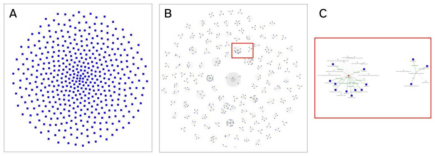
The visualizations below depict a graph of 85K records about Las Vegas businesses, taken from public sources. This data has a 2% duplication rate, although some businesses have up to 14 duplicate records. For this example, we built an entity resolved knowledge graph and then used graph analytics to understand the results. This was quick to run and visualize.
By applying entity resolution to knowledge graphs, organizations are able to make better decisions from their enterprise data, be more competitive, reduce fraud, and service customers better. Many organizations struggle with getting entity resolution into their graph. But it doesn’t have to be hard anymore.
Here’s how you can do this too.
Tutorial overview
This hands-on tutorial in Python demonstrates the integration of Senzing and Neo4j to construct an entity resolved knowledge graph. The code is simple to download and easy to follow and presented so you can try it with your own data.
Here are the steps we will go through to create your entity resolved knowledge graph, with an estimated project time of 35 minutes:
- Use three datasets about Las Vegas area businesses: 85K records, 2% duplicates.
(10 minutes) - Run entity resolution in Senzing to resolve duplicate business names and addresses.
(15 minutes) - Parse the exported results to construct a knowledge graph in Neo4j.
(5 minutes) - Analyze and visualize the entity resolved knowledge graph.
(5 minutes)
We’ll walk through example code based on Neo4j Desktop, using the Graph Data Science (GDS) library to run Cypher queries on the graph, preparing data for downstream analysis and visualizations with Jupyter, Pandas, Seaborn, and PyVis.
In this tutorial, we’ll work in two environments. The configuration and coding are at a level that should be comfortable for most people working in data science. You’ll need to have familiarity with how to:
- Install a desktop/laptop application.
- Clone a public repo from GitHub.
- Launch a server in the cloud.
- Use simple Linux command lines.
- Write some code in Python.
Cloud computing budget: running a cloud instance for Senzing in this tutorial cost a total of $0.04 USD.
Knowledge graph fundamentals
Stop missing hidden patterns in your connected data. Learn graph data modeling, querying techniques, and proven use cases to build more resilient and intelligent applications.
Neo4j environment setup
Neo4j provides native graph storage, graph data science, power graph algorithms and machine learning, analytics, visualization, and so on – with enterprise-grade security controls to scale transactional and analytic workloads. First released in 2010, Neo4j developed and pioneered the use of Cypher, which is a declarative graph query language for labeled property graphs.
Graphs help us understand relationships – unlike relational databases, data warehouses, data lakes, data lakehouses, etc., that tend to emphasize facts.
In Cypher, like the English language, nouns are nodes (aka, entities) in a graph, while verbs are the relationships connecting entities. Cypher defines labels on nodes, in the English language. These categories determine whether proper nouns are a person, place, or thing – and so on. Cypher also defines properties for both nodes and relations, which are adjectives in the English language. The expressiveness of Cypher queries enables building data analytics applications with 10x less code than comparable apps in SQL.
To start coding, let’s set up a Neo4j Desktop application, beginning with the download instructions for your desktop or laptop. There are multiple ways to get started with Neo4j, though Desktop provides a quick way to start with the features we’ll need. It’s available on Mac, Linux, and Windows.
Once the download completes, follow the instructions to install the Desktop application and register to obtain an activation key. Open the application and copy/paste the activation key.
Next, we must create a new project and a database and give it a password. Here are the settings we’ll use:
- Project:
Entity Resolution(our setting, not needed for credentials) - Database:
Senzing(our setting, not needed for credentials) - DBMS:
neo4j(default value, not changed) - Username:
neo4j(default value, not changed) - Password:
uSIv!RFx0Dz(our setting, randomly generated)
We also need to select a Neo4j version – here, we’ll use 5.17.0, which is recent at the time of this writing.
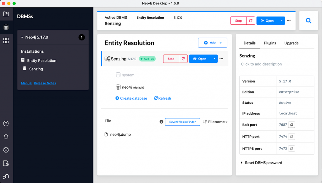
Click on the newly created database, and a right-side panel will display settings and administrative links – as shown in the “Neo4j Desktop” figure. Click on the Plugin link, open the Graph Data Science Library drop-down, then install the GDS plugin. We’ll use the GDS library to access Neo4j through Python code.
Click on the Start button. The GDS plugin will be in place, and local service endpoints for accessing the graph database should be ready. Then click on the Details link and find the port number for the Bolt protocol. In our example, 7687 is the Bolt port number.
Next, open a browser window to our GitHub public repo to download the code for this tutorial.
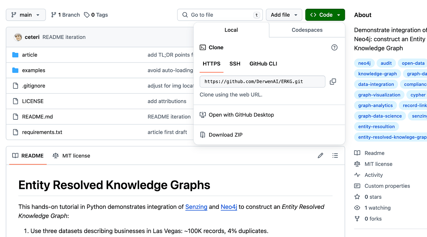
Clone the repo by copying its URL from GitHub, shown in the “Clone public repo from GitHub” figure. Use the following steps to use this cloned repo as the working directory on your desktop/laptop for this tutorial:
After connecting to the working directory, create a file called .env, which provides the credentials (Bolt URL, DBMS, username, password) needed to access the database in Neo4j Desktop through Bolt:
Neo4j Desktop provides many useful tools, including a browser for exploring your graph database and running Cypher queries, and the Bloom data visualization tool. You can also export and import “dumps” of your database on disk, to manage backups.
Neo4j is good to go! For the rest of this tutorial, keep this Neo4j Desktop application running in the background. We’ll access it through the Python API and the Graph Data Science (GDS) library using Python code. To learn more about these libraries, see:
- https://neo4j.com/docs/python-manual/current/install/
- https://github.com/neo4j/graph-data-science-client
- https://neo4j.com/docs/graph-data-science/current/
Installing the input datasets
We’ll work with three datasets to run entity resolution and build a knowledge graph. To start, let’s set up a Python environment and install the libraries we’ll need. Then we can run code examples inside Jupyter notebooks. We show the use of Python 3.11 here, although other recent versions of Python should work well too.
Set up a virtual environment for Python and load the required dependencies:
This tutorial uses several popular libraries which are common in data science work:
Now launch Jupyter:
JupyterLab should automatically open in the browser. Otherwise, open http://localhost:8888/lab in a new browser tab. Then run the datasets.ipynb notebook.
First, we need to import the Python library dependencies required for the code we’ll be running:
Let’s double-check the watermark trace, in case anyone needs to troubleshoot dependencies on their system:
For example, the results should look like:
Python, Jupyter, GDS, Pandas, and friends are good to go! Let’s leverage these to explore the datasets we’ll be using.
In this tutorial, we’ll use three datasets that describe business info – names, addresses, plus other details, depending on the dataset:
- SafeGraph: Places of Interest (POI).
- US Department of Labor: Wage and Hour Compliance Action Data (WHISARD).
- US Small Business Administration: PPP Loans over $150K (PPP).
In this tutorial, we’re using versions of these datasets, which have been constrained to businesses within the Las Vegas metropolitan area. We also include a DATA_SOURCE column in each dataset, used to load and track records in Senzing later.
Download these datasets (snapshots in time, to make the tutorial results consistent).
For the sake of brevity, we’ve shortened their file names to poi.json, dol.json, and ppp.json, respectively.
Let’s explore each of these datasets. To help do this, we’ll define a utility function sample_df() to show a subset of columns in a Pandas DataFrame object:
Now we’ll load the Places of Interest (POI) from SafeGraph:
Note that we’ve added a name column, as a copy of LOCATION_NAME_ORG. This will get used later for loading records into Neo4j and graph visualization, it is not part of the data that gets loaded into Senzing.
Taking a look at the column names, the DATA_SOURCE, RECORD_ID, and RECORD_TYPE columns are needed by Senzing to identify unique records, then other columns related to names or addresses will also be used during entity resolution:
See the SafeGraph docs for detailed descriptions of the data in each of these columns.
Let’s check out a few key columns:
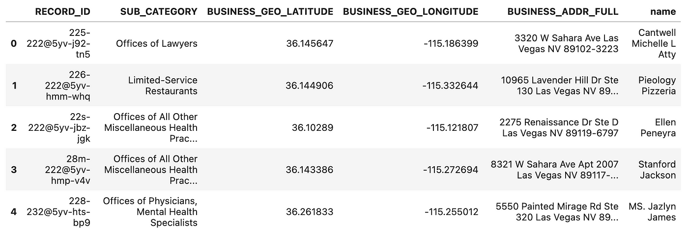
From this sample, note the unique values in RECORD_ID plus the business names and addresses. The business category values could be used to add structure to the knowledge graph – as a kind of taxonomy. The latitude and longitude geo-coordinates could also help us convert the results of graph queries into map visualizations.
Let’s analyze the data values in these columns:
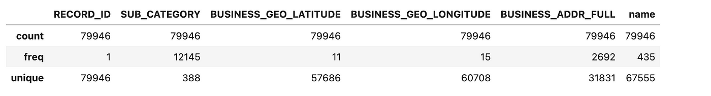
We’ve got 79,946 records to work with, and their RECORD_ID values are all unique. There are 388 different kinds of business categories, which could be fun to visualize.
Take note, there are 67,555 unique values of business names and 31,831 unique values in the BUSINESS_ADDR_FULL column. Are these duplicate entities, businesses with many locations (e.g., BurgerKing), or many businesses at the same location (e.g., Gallery Mall)? Clearly, we’ll need to run entity resolution to find out!
Next, let’s load the Wage and Hour Compliance Action Data (WHISARD) from the US Department of Labor:
The Department of Labor publishes a data dictionary on its website, which describes each of the fields.
Looking at the column names, again, we have DATA_SOURCE, RECORD_ID, plus business names and address info, followed by lots of DoL compliance data about hourly workers:
Let’s check some of the more interesting columns:
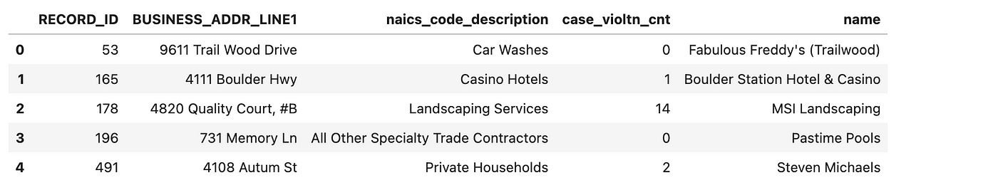
Again we have unique record IDs, business names and addresses, then also some NAICS business classification info – which the POI dataset also includes. The case_violtn_cnt column provides a count of compliance violation cases, and that could be interesting to use in graph queries later.
Analyzing the data values in this sample:
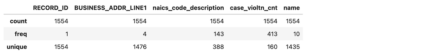
The record IDs are unique, and there’s overlap among business names and addresses. However, we only have 1,554 records here, so not every resolved entity will link to the Department of Labor compliance information. But we’ll make use of what we’ve got.
Next, we’ll load the PPP Loans over $150K (PPP) dataset for Las Vegas, which comes from the US Small Business Administration:
This dataset adds more details from US federal open data about each business, based on their PPP loans (if any) during the Covid-19 pandemic:
Let’s take a look at a sample:
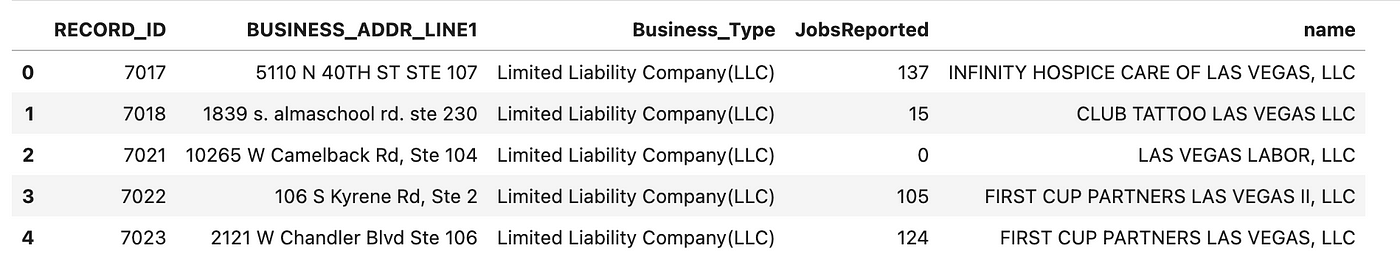
Great, here we get more info about business types, and we also get new details about employment. Both of these could complement the DoL WHISGARD dataset.
Analyzing data values in this sample:
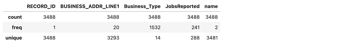
Again, the record IDs are unique, and there’s overlap among business names and addresses. We have 3,488 unique records, so not all resolved entities will likely have PPP data. There are 14 different business types, which could also help add structure to our knowledge graph.
Now that we have our three datasets ready, let’s load their records into Neo4j. First, we need to use our credentials – which were stored in the .env local file in our working directory – to create a GDS instance to connect to our Senzing graph database running in Neo4j Desktop:
To prepare to add structure to our graph, we’ll add a constraint to ensure the uniqueness of nodes representing input data records:
Next, we’ll define utility methods to clean and prep the data from our datasets:
Then we can load records into Neo4j. The Cypher clause UNWIND turns a converted DataFrame (e.g., the $rows parameter) into individual rows.
Combined with a sub-query, this clause functions like a batch load. Using mini-batches of 10,000 runs much faster than loading rows by iterating over them one transaction at a time.
Now we use this approach to load the three datasets:
Boom! There are now nearly 85,000 records represented as nodes in Neo4j. However, these nodes have no connections. Clearly there was overlap among the business names and addresses, but we don’t have any of them resolved as entities yet. We’ll fix that next, and then see how this data starts becoming a graph.
Note that the Neo4j node for each loaded record has:
- A
:Recordlabel to distinguish from other kinds of nodes. - A unique ID
uid, which ties back to the input dataset records. - Properties to represent other fields from the datasets.
Installing the Senzing library
Senzing provides a purpose-built AI for real-time entity resolution, a 6th generation industrial-strength engine, making entity resolution for developers easy. A motto at the company is “We sell transmissions, not cars.” To be clear, everything about this technology is laser-focused on providing speed, accuracy, and throughput for the best quality ER available – connecting the right data to the right person, in real-time. The company’s expertise in this field is stellar: the engineers on the team have been working together on this technology on average for more than 20 years, often in extreme production use cases.
Note that the Senzing binary is downloaded and runs entirely local on your cloud or on-prem infrastructure. Also, check out https://github.com/Senzing on GitHub, where you can find more than 30 public repos. You can download and get running right away, with a free license for up to 100,000 records. This scales from the largest use cases all the way down to running on a laptop. You can run from Docker containers available as source on GitHub or images on Docker Hub, or develop code using API bindings for Java and Python.
There are multiple convenient ways to get started with Senzing. Production use cases typically develop a Java or Python application which calls the Senzing API running in a container – as a microservice. For the purposes of this tutorial, we’ll run Senzing on a Linux server in a cloud. The steps to access via a Linux command line are simple, and there’s already proof-of-concept demo code available in Python. We can simply import our datasets to the cloud server, then export the ER results from it using file transfer.
We’ll follow steps from the Quickstart Guide, based on using Debian (Ubuntu) Linux. First, we need to launch a Linux server using one of the popular cloud providers (pick one, any one) which is running an Ubuntu 20.04 LTS server with 4 vCPU and 16 GB memory. Be sure to configure enough memory.
Now download the Senzing installer image and run it:
Depending on the Linux distribution and version, the last two steps may require installing libssl1.1 before they can run correctly. Most definitely, the apt installer utility will let you know through error messages if this is the case! Instructions are described in the question-answer on StackOverflow.
Now we’re ready to install the Senzing library.
This installation will be located in the /opt/senzing/data/current directory. Senzing is good to go!
Next, we’ll use a sample data loader for Senzing called G2Loader which is written in Python. This application calls the Senzing APIs, the same APIs you would use in production use cases. Check the code if you’re curious about its details, and see other examples on GitHub.
Let’s create a project for G2Loader named ~/senzing in the user home directory:
Then set up the configuration:
Next, we need to upload the three datasets to the cloud server. For example, we could transfer these files through a bucket in the cloud provider’s storage grid. For this tutorial, we’ve placed these files in the lv_data subdirectory:
Next, prepare to load these datasets as Senzing data sources:
It may be simpler to run the ./python/G2ConfigTool.py configuration tool interactively, rather than type the command shown above in the shell prompt.
Now we’re ready to run ER in Senzing. We’ll specify using up to 16 threads to parallelize the input process. This way, the following steps take advantage of multiple CPU cores and are completed within a few minutes:
The resolved entities can now be exported to a JSON file using one line:
To explore these results manually, note that the export.json file has one dictionary per line. We can run a simple command line pipe to “pretty-print” the first resolved entity:
We won’t print the full details here, but the output should start with something like:
Transfer the export.json local file from the cloud server back to your desktop/laptop and move it into the working directory.
Done and done! That was quick. To launch a cloud server, install Senzing, load three datasets, run entity resolution, then download results: less than one hour. This cost a total of $0.04 USD to run (depending on your cloud server configuration). Of course, you could simply run a Docker container locally to call Senzing as a microservice – but there’s so much less to observe and discuss.
Building an entity resolved knowledge graph
Return to the Jupyter browser tab and open the graph.ipynb notebook. Again, we need to import Python library dependencies:
Then check the watermark trace:
We’re ready to parse the entity resolution results from Senzing, using them to construct a knowledge graph in Neo4j. The entities and relations derived from ER will get used to link the structure initially in our KG.
Let’s define a dataclass to represent the parsed results from ER as Python objects:
Now let’s parse the JSON data from the export – in the export.json file downloaded from the cloud server. We’ll build a dictionary of entities indexed by unique identifiers, keeping track of both the “resolved” and “related” records for each entity to use later when constructing the KG:
On a not-so-new Mac laptop, this ran in about 3 seconds.
To finish preparing the input data for resolved entities, let’s make a quick traversal of the record linkage and set a flag has_ref for “interesting” entities that will have relations in the graph to visualize.
Let’s look at one of these parsed entity records:
We have unique IDs for entities and records, so we can link these as relations in the graph data. We’ve also got interesting info about how the record matches were determined, which could be used as properties on the graph relations.
Next, we create a GDS instance to connect to the Neo4j graph database, then create a constraint for the :Entity nodes:
Now it’s simple to load the entities as nodes:
We’ll connect each entity with its resolved records:
Similarly, we’ll connect each entity with its related entities, if any:
Now let’s look at the schema that we’ve built so far in our graph database – in other words, the structure of our KG so far. In the Browser window of Neo4j Desktop, run the following Cypher command at the neo4j$ prompt to visualize the database schema:
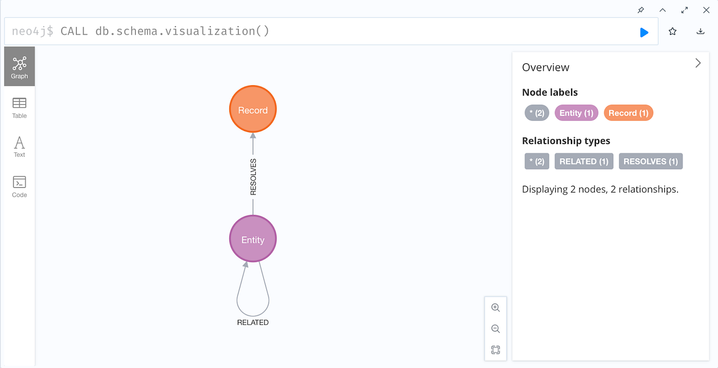
This is starting to resemble a knowledge graph! Let’s dig into more details.
Since we’re trying to link records across the three datasets, it’d be helpful to measure how much the process of ER has consolidated records among the input datasets. In particular, it’d be helpful to understand:
- Total number of entities.
- Number of entities with linked reference (should be 100%).
- Number of linked records per entity.
- Number of related entities per entity.
In the Jupyter browser tab, open the impact.ipynb notebook. We’ll load the imports, check the watermark, and create a GDS instance – just as before. Then we’ll leverage GDS to run analysis with Pandas, Seaborn, etc.:
The results show:
Great, 100% of the input records have been resolved as entities – as expected. An average rate of ~2% duplicates was detected among these records.
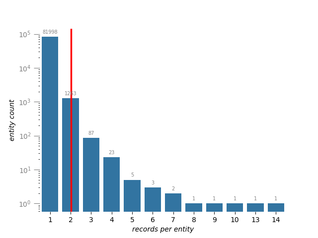
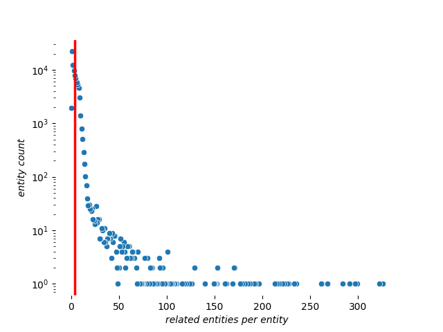
Let’s check the distributions for resolved records and related entities:
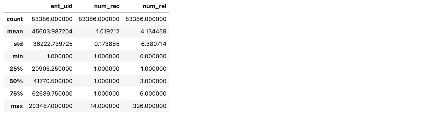
The mean count of resolved records per entity is ~1.02 and the mean count of related entities is ~4.13 per entity. Note that some entities have more than 300 related entities.
Let’s run more detailed statistical analysis for the resolved entities. We’ll repeat the following graph data science sequence of steps to explore this linking:
- Run a Cypher query in Neo4j using GDS.
- Collect query results as a Pandas
DataFrameobject. - Use Seaborn to analyze and visualize the results.
Let’s use the PyVis library in Python to visualize relations in our KG. First we’ll show the unconnected data graph of input records – filtering out the business entities which don’t have duplicates so we can compare the impact of ER visually:
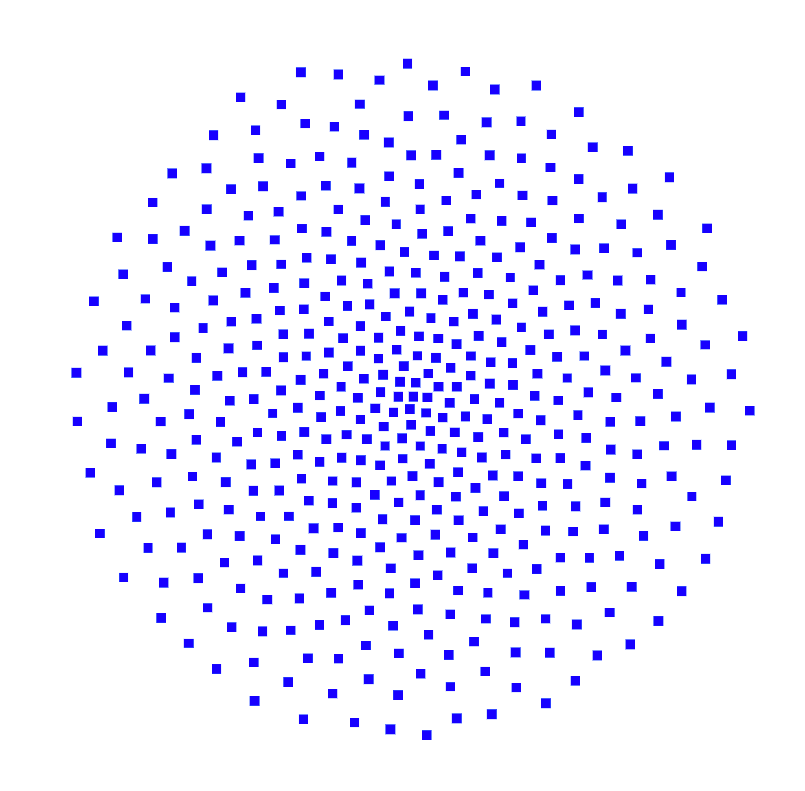
This visualization above shows just the records from the three datasets loaded into Neo4j. At this stage, we could say this is a data graph, even though it doesn’t have any links yet. The distinction is that data graphs are at a lower level of organization than knowledge graphs: they provide more details, especially about provenance, but lack the semantics for a KG.
Now we’ll illustrate the convergence of dataset records achieved through entity resolution:
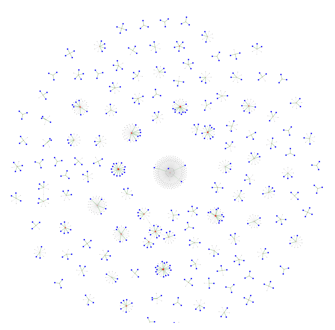
And voilà – our graph begins to emerge! The full HTML+JavaScript file is large and may take a few minutes to load. You can also view these results by loading the big_vegas.2.html file in your web browser.
Here the red stars are entities, while the blue squares are input data records. Notice these clusters, some of which have a dozen or more records linked to the same entity.
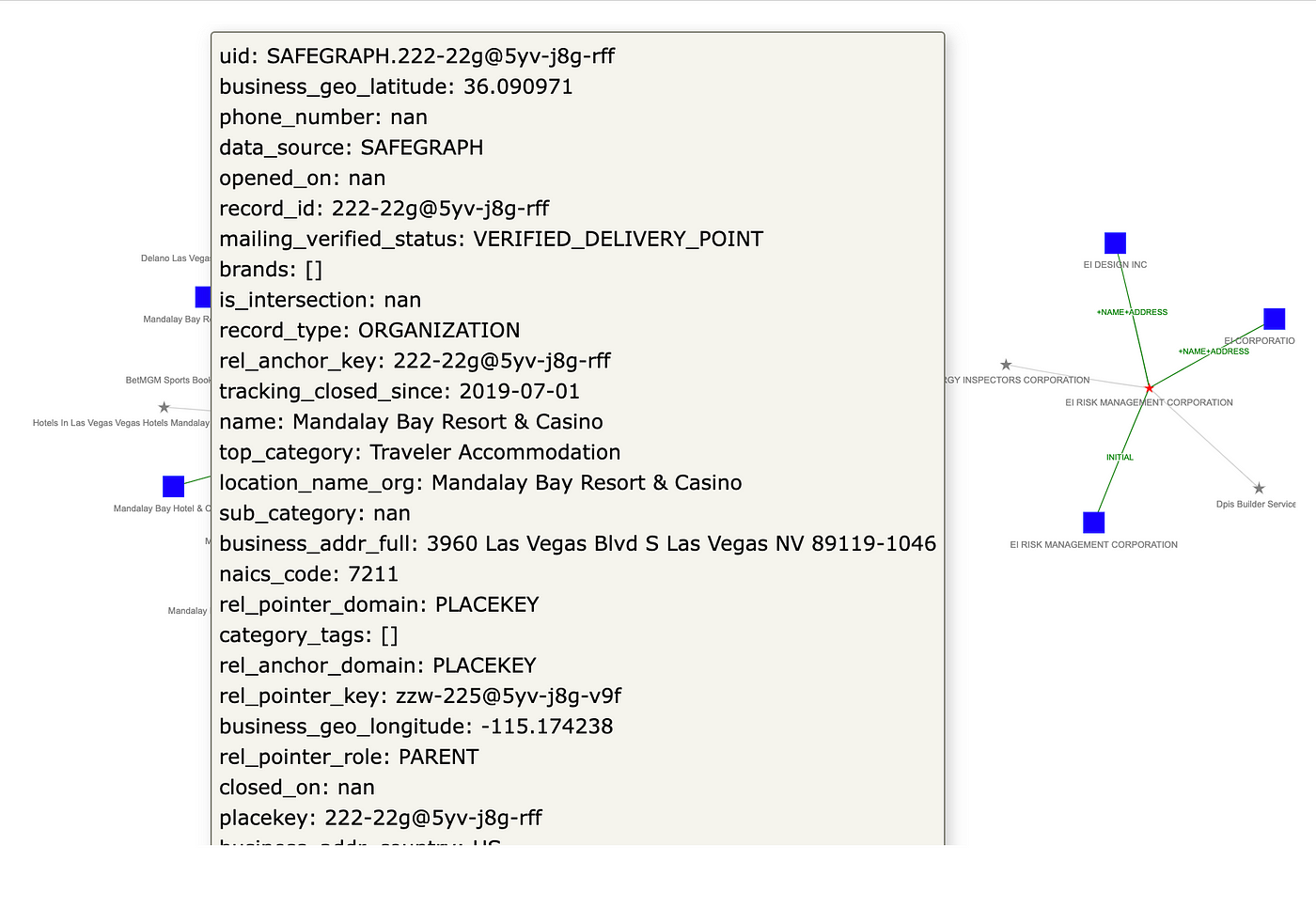
Let’s zoom into this graph just above the center of the visualization. Notice the MATCH_KEY labels on the :RESOLVES relationships, which describe the decisions during entity resolution:

Based on how we’ve set the title attribute for :Record nodes, we can “flyover” a node to see all the properties for that record:
Going back to Neo4j Desktop, from the left sidebar menu, select Neo4j Bloom, which provides even more powerful means for interactive graph visualization and analysis.
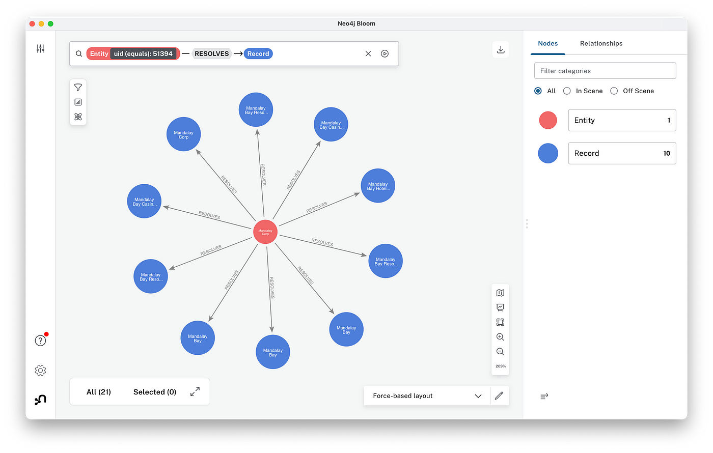
Click the query box at the top-left of the Bloom window to describe the relations you want to explore. There’s a panel on the right which can be used to specify properties, colors, shapes, and so on. The figure above shows the (:Entity)-[:RESOLVES]->(:Record) relation. Zooming into this graph, we see 10 records which have been resolved as the entity representing Mandalay, with duplicates mostly coming from the DoL WHISARD dataset.
Some of the most powerful features of entity resolution in Senzing are where specific entities can be audited and updated; similarly the power of a knowledge graph in Neo4j is to be able to navigate quickly and conveniently through the resolve records to identify cases which require updates. Downstream applications based on your ERKG, such as AI use cases, will appreciate having the corrected entity data.
Summary
To recap, here’s a list of what we’ve just accomplished:
- Installed Neo4j Desktop and cloned a public GitHub repo locally to get code for this tutorial.
- Loaded three datasets about businesses in Las Vegas: records for 85K business, with 2% duplicates based on slight variations in names and addresses.
- Used Pandas to review the input data, then loaded records into Neo4j – at this point as unconnected nodes and properties.
- Installed Senzing on a Linux cloud server instance, uploaded the three datasets, and ran entity resolution.
- Exported the ER results back to the desktop/laptop, then parsed the JSON and loaded entities into Neo4j.
- Connected the entities with the input records.
- Used Seaborn to analyze the difference that ER makes, quantitatively and in histograms.
- Used PyViz to build interactive visualizations of the “before” data graph versus the “after” entity resolved knowledge graph.
- Also thought a lot along the way about how to mine this data to build even more structure into the KG, leveraging it with GraphRAG to build a custom LLM application that answers burning questions about Las Vegas.
Learning resources
Imagine the questions we could answer when you pair an entity resolved knowledge graph with LLM applications. For example, “Where’s a pizza restaurant with a large number of employees and no history of compliance violations, located near a bike shop and a cinema?”
Check out Using a Knowledge Graph to Implement a RAG Application by Tomaz Bratanic to learn more about GraphRAG and ERKGs in AI applications. Stay tuned for our next tutorial here, too.
Also, check this highly recommended video for a demonstration of how to use entity resolved knowledge graphs in practice, Analytics on Entity Resolved Knowledge Graphs by Mel Richey.
For details about the Senzing AI and how entity resolution works, see:
- What Is Entity Resolution? Entity Resolution Defined
- Entity Resolution Explained Step by Step
- Entity Resolution: Insights and Implications for AI Applications
- Benefits of Entity Resolved Knowledge Graphs
To learn more about Neo4j, there’s an incredible developer community, with many resources available online. Check out https://github.com/neo4j on GitHub for more than 70 public repos supporting a wide range of graph technologies. There’s an excellent introduction in the recent Intro to Neo4j video. Also, check the many online courses, certification programs, and other resources at GraphAcademy.
How to build a knowledge graph
Learn the basics of graph data modeling, how to query, and top use cases that use highly interconnected data.
Share Article


Explore
Related Articles
Hybrid Search in Neo4j: Full-Text, Vectors, and Graph Topology with Cypher