Exploring Fraud Detection With Neo4j & Graph Data Science – Part 3

Data Science Product Specialist, Neo4j
5 min read
In parts 1 & 2 of this series, we explored the graph and identified high risk fraud communities. At this stage, we may want to expand beyond our business logic to automatically identify other users that are suspiciously similar to the fraud risks already identified. Neo4j and GDS makes it simple to triage and recommend such suspect users in a matter of seconds. We can leverage both centrality and similarity algorithms for this.
The technical resources to reproduce this analysis and the analysis in all other parts of this series are contained in this GitHub repository, which includes an iPython notebook and link to the dataset.
Using Weighted Degree Centrality to Recommend Potential High Risk Accounts
We can quickly and easily generate a ranked list of suspicious user accounts with weighted degree centrality. Specifically, we can calculate the degree centrality of users in respect to their identifiers (Devices, Cards, and IPs) weighted by the fraudRiskRatio values we made in part 2. In this case, a simple Cypher query suffices.
gds.run_cypher('''
    MATCH(f:FraudRiskUser)-[:HAS_CC|HAS_IP|USED]->(n)
    WITH DISTINCT n
    MATCH(u:User)-[:HAS_CC|HAS_IP|USED]->(n) WHERE NOT u:FraudRiskUser
    WITH left(u.guid,8) as uid,
        sum(n.fraudRiskRatio) AS totalIdFraudRisk,
        count(n) AS numberFraudRiskIds
    WITH uid, totalIdFraudRisk,
        numberFraudRiskIds,
        totalIdFraudRisk/toFloat(numberFraudRiskIds) AS averageFraudIdRisk
    WHERE averageFraudIdRisk >= 0.25
    RETURN uid, totalIdFraudRisk, numberFraudRiskIds, averageFraudIdRisk
    ORDER BY totalIdFraudRisk DESC LIMIT 10
''')
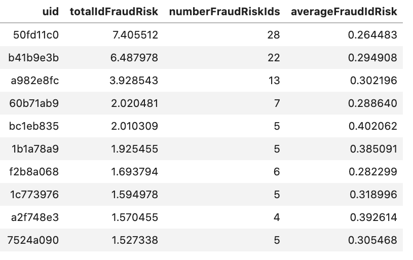
Users in the above result list are sorted by how much identifying information they share with previously labeled fraud risks, the ones with the most being at the top. Technically speaking, these users are ranked by their total Id fraud risk, which is equal to the sum of the fraudRiskRatios from the Identifiers they are connected to.
In the query, I also implement a limit on the average fraud risk to avoid users that just have a lot of high-degree identifiers (likely proxy IP addresses shared by only a small fraction of fraud risk users). This sort of filtering can be tweaked by use case to get the right balance between total risk vs average risk.
In a real-world fraud detection use case, these results can be triaged by analysts to label more fraud accounts and grow labeled fraud communities.
Using Node Similarity to Expand on Fraud Communities
Simple calculations like weighted degree centrality work well for identifying suspicious users over the whole graph, but what if we are interested in how users are related to a specific fraud risk community or set of communities? Perhaps we hypothesize that communities of fraud risk users are actually bigger than currently represented but we don’t have exact business rules to apply. We can leverage similarity algorithms to help us score and recommend users for this.
GDS offers multiple algorithms for similarity. In this analysis I will focus on the aptly named Node Similarity algorithm — you can read more about it here. Node similarity parallelizes well and is explainable. It identifies pairs of similar nodes based on a straightforward Jaccard similarity calculation. So while other ML-based similarity approaches like FastRP + KNN covered in this post scale well globally on very large graphs, Node Similarity is a good choice where explainability is important and you can narrow down the universe of comparisons to a subset of your data.
Examples of narrowing down include focusing on just single communities, newly added users, or nodes within a specific proximity to a subset of users. In this analysis we will take the third approach, identifying similarity between user accounts using just the Card, Device, and IP address nodes that connect to at least one fraud risk account from part 2.
Below I apply three queries to calculate node similarity. The first query enables the identifier filtering via setting a new label on the Card, Device, and IP address nodes that connect to fraud risk accounts. The first query also weights relationships by the inverse of degree centrality, essentially downplaying the importance of identifiers proportional to the number of other users they connect to.
This is important as some identifiers, particularly IP addresses, can connect to hundreds or thousands of users, in which case the identifier may be very generic (like a proxy IP address) and not as relevant to true user identity. The second and third query project the graph and write relationships back to the database with a score to represent similarity strength between user node pairs. You will notice that I use a similarity cutoff of 0.01 in the third query, which is intended to rule out weak associations and keep the similarities relevant.
gds.run_cypher('''
    MATCH(f:FraudRiskUser)-[:HAS_CC|HAS_IP|USED]->(n)
    WITH DISTINCT n
    MATCH(n)<-[r:HAS_CC|HAS_IP|USED]-(u)
    SET n:FraudSharedId
    SET r.inverseDegreeWeight = 1.0/(n.degree-1.0)
    RETURN count(DISTINCT n)
''')

count(DISTINCT n)
18182

g, _ = gds.graph.project('similarity-projection', ['User', 'FraudSharedId'],
        ['HAS_CC', 'USED', 'HAS_IP'], relationshipProperties=['inverseDegreeWeight'])

_ = gds.nodeSimilarity.write(g, writeRelationshipType='SIMILAR_IDS', writeProperty='score',
        similarityCutoff=0.01, relationshipWeightProperty='inverseDegreeWeight')
g.drop()
From there, we can run a Cypher query to rank users by how similar they are to known fraud risk communities.
gds.run_cypher('''
    MATCH (f:FraudRiskUser)
    WITH f.wccId AS componentId, count(*) AS numberOfUsers, collect(f) AS users
    UNWIND users AS f
    MATCH (f)-[s:SIMILAR_IDS]->(u:User)
    WHERE NOT u:FraudRiskUser AND numberOfUsers > 2
    RETURN u.guid AS userId, sum(s.score) AS totalScore,
        collect(DISTINCT componentId) AS closeToCommunityIds
    ORDER BY totalScore DESC
''')
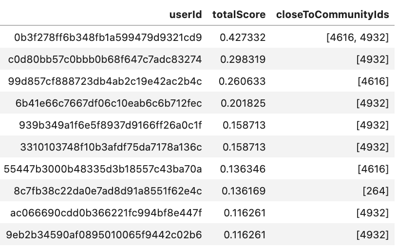
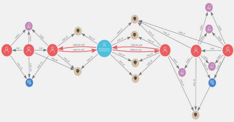
Let’s take a look at the first user in the list, user 0b3f278f..., in Neo4j Bloom. This user account seems interesting in the sense that they connect to two different communities.
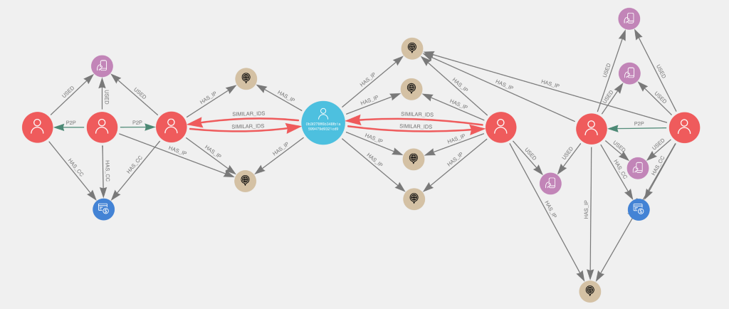
You can see how this user connects to the two fraud risk communities and how the similarity relationships were based on shared IP addresses. This user seems to act as a sort of bridge between the two communities, suggesting not only that the user is likely part of the fraud communities but also that the two communities may actually reflect one-in-the same.
Conclusions
Overall, centrality and similarity metrics like these are fast and easy to implement with Neo4j and GDS. They can help advance your Data Science approach by introducing automated and semi-supervised processes to assist in targeted triage and identification of suspicious user accounts based on previously labeled data. In the next part, we will show you how to take fraud detection even further with machine learning.
Here’s your key to the whole series:
Share Article


Explore
Related Articles

Mastering Fraud Detection With Temporal Graph Modeling

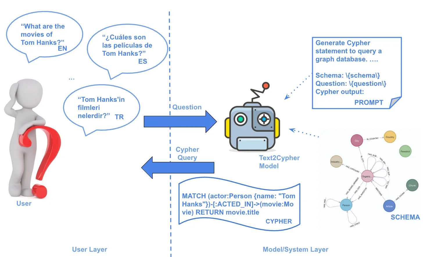
Text2Cypher Across Languages: Evaluating Foundational Models Beyond English