Label Propagation
Glossary
- Directed
-
Directed trait. The algorithm is well-defined on a directed graph.
- Undirected
-
Undirected trait. The algorithm is well-defined on an undirected graph.
- Heterogeneous nodes
-
Heterogeneous nodes fully supported. The algorithm has the ability to distinguish between nodes of different types.
- Heterogeneous relationships
-
Heterogeneous relationships fully supported. The algorithm has the ability to distinguish between relationships of different types.
- Weighted relationships
-
Weighted trait. The algorithm supports a relationship property to be used as weight, specified via the relationshipWeightProperty configuration parameter.
- Node properties
-
Node properties trait. The algorithm makes use of node properties.
- CPU
-
The algorithm runs on CPU compute pools.
- GPU
-
The algorithm runs on GPU compute pools.
Introduction
The Label Propagation algorithm (LPA) is a fast algorithm for finding communities in a graph. It detects these communities using network structure alone as its guide, and doesn’t require a pre-defined objective function or prior information about the communities.
LPA works by propagating labels throughout the network and forming communities based on this process of label propagation.
The intuition behind the algorithm is that a single label can quickly become dominant in a densely connected group of nodes, but will have trouble crossing a sparsely connected region. Labels will get trapped inside a densely connected group of nodes, and those nodes that end up with the same label when the algorithms finish can be considered part of the same community.
The algorithm works as follows:
-
Every node is initialized with a unique community label (an identifier).
-
These labels propagate through the network.
-
At every iteration of propagation, each node updates its label to the one that the maximum numbers of its neighbours belongs to. Ties are broken arbitrarily but deterministically.
-
LPA reaches convergence when each node has the majority label of its neighbours.
-
LPA stops if either convergence, or the user-defined maximum number of iterations is achieved.
As labels propagate, densely connected groups of nodes quickly reach a consensus on a unique label. At the end of the propagation only a few labels will remain - most will have disappeared. Nodes that have the same community label at convergence are said to belong to the same community.
One interesting feature of LPA is that nodes can be assigned preliminary labels to narrow down the range of solutions generated. This means that it can be used as semi-supervised way of finding communities where we hand-pick some initial communities.
For more information on this algorithm, see:
Syntax
This section covers the syntax used to execute the Label Propagation algorithm.
CALL Neo4j_Graph_Analytics.graph.label_propagation(
  'CPU_X64_XS',                    (1)
  {
    ['defaultTablePrefix': '...',] (2)
    'project': {...},              (3)
    'compute': {...},              (4)
    'write':   {...}               (5)
  }
);| 1 | Compute pool selector. |
| 2 | Optional prefix for table references. |
| 3 | Project config. |
| 4 | Compute config. |
| 5 | Write config. |
| Name | Type | Default | Optional | Description |
|---|---|---|---|---|
computePoolSelector |
String |
|
no |
The selector for the compute pool on which to run the Label Propagation job. |
configuration |
Map |
|
no |
Configuration for graph project, algorithm compute and result write back. |
The configuration map consists of the following three entries.
| For more details on below Project configuration, refer to the Project documentation. |
| Name | Type |
|---|---|
nodeTables |
List of node tables. |
relationshipTables |
Map of relationship types to relationship tables. |
| Name | Type | Default | Optional | Description |
|---|---|---|---|---|
resultProperty |
String |
|
yes |
The node property that will be written back to the Snowflake database. |
nodeWeightProperty |
String |
|
yes |
The name of a node property that contains node weights. |
relationshipWeightProperty |
String |
|
yes |
Name of the relationship property to use as weights. If unspecified, the algorithm runs unweighted. |
seedProperty |
String |
|
yes |
Used to set the initial community for a node. The property value needs to be a non-negative number. |
maxIterations |
Integer |
|
yes |
The maximum number of iterations to run. |
| For more details on below Write configuration, refer to the Write documentation. |
| Name | Type | Default | Optional | Description |
|---|---|---|---|---|
nodeProperty |
String |
|
yes |
The node property that will be written back to the Snowflake database. |
Examples
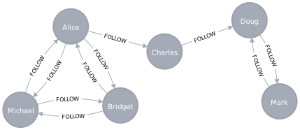
In this section we will show examples of running the Label Propagation algorithm on a concrete graph. The intention is to illustrate what the results look like and to provide a guide on how to make use of the algorithm in a real setting. We will do this on a small social network graph of a handful of nodes connected in a particular pattern. The example graph looks like this:
CREATE OR REPLACE TABLE EXAMPLE_DB.DATA_SCHEMA.USERS (NODEID VARCHAR, SEED NUMBER);
INSERT INTO EXAMPLE_DB.DATA_SCHEMA.USERS VALUES
  ('Alice', 42),
  ('Bridget', 42),
  ('Charles', 42),
  ('Doug', NULL),
  ('Mark', NULL),
  ('Michael', NULL);

CREATE OR REPLACE TABLE EXAMPLE_DB.DATA_SCHEMA.LINKS (SOURCENODEID VARCHAR, TARGETNODEID VARCHAR, WEIGHT FLOAT);
INSERT INTO EXAMPLE_DB.DATA_SCHEMA.LINKS VALUES
  ('Alice',   'Bridget', 1),
  ('Alice',   'Charles', 1),
  ('Charles', 'Bridget', 1),
  ('Alice',   'Doug',    5),
  ('Mark',    'Doug',    1),
  ('Mark',    'Michael', 1),
  ('Michael', 'Mark',    1);
This graph represents six users, some of whom follow each other.
Besides a name property, each user also has a seed property.
The seed property represents a value in the graph used to seed the node with a label.
For example, this can be a result from a previous run of the Label Propagation algorithm.
In addition, each relationship has a weight property.
With the node and relationship tables in Snowflake we can now project it as part of an algorithm job. In the following examples we will demonstrate using the Label Propagation algorithm on this graph.
Run job
Running a Label Propagation algorithm job involves three steps: Project, Compute and Write.
To run the query, there is a required setup of grants for the application, your consumer role and your environment. Please see the Getting started page for more on this.
We also assume that the application name is the default Neo4j_Graph_Analytics. If you chose a different app name during installation, please replace it with that.
CALL Neo4j_Graph_Analytics.graph.label_propagation('CPU_X64_XS', {
    'defaultTablePrefix': 'EXAMPLE_DB.DATA_SCHEMA',
    'project': {
        'nodeTables': [ 'USERS' ],
        'relationshipTables': {
            'LINKS': {
                'sourceTable': 'USERS',
                'targetTable': 'USERS'
            }
        }
    },
    'compute': {
    },
    'write': [{
        'nodeLabel': 'USERS',
        'outputTable': 'USERS_COMMUNITY'
    }]
});| JOB_ID | JOB_STATUS | JOB_START | JOB_END | JOB_RESULT |
|---|---|---|---|---|
job_b1e167d1f8e64e229e4af0188072c61e |
SUCCESS |
2026-05-11 10:49:49.953 |
2026-05-11 10:49:58.546 |
 {
  "label_propagation_1": {
    "communityCount": 2,
    "communityDistribution": {
      "max": 3,
      "mean": 3,
      "min": 3,
      "p1": 3,
      "p10": 3,
      "p25": 3,
      "p5": 3,
      "p50": 3,
      "p75": 3,
      "p90": 3,
      "p95": 3,
      "p99": 3,
      "p999": 3
    },
    "computeMillis": 35,
    "configuration": {
      "concurrency": 2,
      "consecutiveIds": false,
      "maxIterations": 10,
      "nodeLabels": [
        "*"
      ],
      "nodeWeightProperty": null,
      "relationshipTypes": [
        "*"
      ],
      "resultProperty": "community",
      "seedProperty": null
    },
    "didConverge": true,
    "ranIterations": 3
  },
  "project_graph_1": {
    "graphName": "snowgraph",
    "nodeCount": 6,
    "nodeLabels": {
      "NODE": {
        "count": 6,
        "nodeId": {
          "dataType": "LONG"
        },
        "properties": {
          "POSTS": {
            "dataType": "LONG"
          },
          "SEED_LABEL": {
            "dataType": "LONG"
          }
        },
        "table": "EXAMPLE_DB.DATA_SCHEMA.USERS"
      }
    },
    "nodeMillis": 340,
    "relationshipCount": 10,
    "relationshipMillis": 931,
    "relationshipTypes": {
      "RELATIONSHIP": {
        "count": 10,
        "direction": "DIRECTED",
        "properties": {
          "WEIGHT": {
            "dataType": "DOUBLE"
          }
        },
        "sourceTable": "EXAMPLE_DB.DATA_SCHEMA.USERS",
        "targetTable": "EXAMPLE_DB.DATA_SCHEMA.USERS"
      }
    },
    "totalMillis": 1271
  },
  "write_node_property_1": {
    "copyIntoTableMillis": 969,
    "nodeLabel": "USERS",
    "nodeProperty": "community",
    "outputTable": "EXAMPLE_DB.DATA_SCHEMA.USERS_COMMUNITY",
    "rowsWritten": 6,
    "stageUploadMillis": 2157,
    "writeMillis": 3320
  }
} |
In the above example we can see that our graph has two communities each containing three nodes.
The default behaviour of the algorithm is to run unweighted, e.g. without using node or relationship weights.
The weighted option will be demonstrated in Weighted
SELECT * FROM EXAMPLE_DB.DATA_SCHEMA.USERS_COMMUNITY;| NODEID | COMMUNITY |
|---|---|
Alice |
1 |
Bridget |
1 |
Charles |
4 |
Doug |
4 |
Mark |
4 |
Michael |
1 |
We use default values for the procedure configuration parameters.
Weighted
The Label Propagation algorithm can also run on weighted graphs.
To tell the algorithm to use the projected relationship weights, set the relationshipWeightProperty configuration parameter.
CALL Neo4j_Graph_Analytics.graph.label_propagation('CPU_X64_XS', {
    'defaultTablePrefix': 'EXAMPLE_DB.DATA_SCHEMA',
    'project': {
        'nodeTables': [ 'USERS' ],
        'relationshipTables': {
            'LINKS': {
                'sourceTable': 'USERS',
                'targetTable': 'USERS',
            }
        }
    },
    'compute': {
        'relationshipWeightProperty': 'WEIGHT'
    },
    'write': [{
        'nodeLabel': 'USERS',
        'outputTable': 'USERS_COMMUNITY_WEIGHTED'
    }]
});| JOB_ID | JOB_STATUS | JOB_START | JOB_END | JOB_RESULT |
|---|---|---|---|---|
job_b198320e023c42d8823da59e1f8ce3d0 |
SUCCESS |
2026-05-11 10:23:29.793 |
2026-05-11 10:23:39.255 |
 {
  "label_propagation_1": {
    "communityCount": 2,
    "communityDistribution": {
      "max": 4,
      "mean": 3,
      "min": 2,
      "p1": 2,
      "p10": 2,
      "p25": 2,
      "p5": 2,
      "p50": 2,
      "p75": 4,
      "p90": 4,
      "p95": 4,
      "p99": 4,
      "p999": 4
    },
    "computeMillis": 85,
    "configuration": {
      "concurrency": 2,
      "consecutiveIds": false,
      "maxIterations": 10,
      "nodeLabels": [
        "*"
      ],
      "nodeWeightProperty": null,
      "relationshipTypes": [
        "*"
      ],
      "relationshipWeightProperty": "WEIGHT",
      "resultProperty": "community",
      "seedProperty": null
    },
    "didConverge": true,
    "ranIterations": 4
  },
  "project_graph_1": {
    "graphName": "snowgraph",
    "nodeCount": 6,
    "nodeLabels": {
      "NODE": {
        "count": 6,
        "nodeId": {
          "dataType": "LONG"
        },
        "properties": {
          "POSTS": {
            "dataType": "LONG"
          },
          "SEED_LABEL": {
            "dataType": "LONG"
          }
        },
        "table": "EXAMPLE_DB.DATA_SCHEMA.USERS"
      }
    },
    "nodeMillis": 403,
    "relationshipCount": 10,
    "relationshipMillis": 810,
    "relationshipTypes": {
      "RELATIONSHIP": {
        "count": 10,
        "direction": "DIRECTED",
        "properties": {
          "WEIGHT": {
            "dataType": "DOUBLE"
          }
        },
        "sourceTable": "EXAMPLE_DB.DATA_SCHEMA.USERS",
        "targetTable": "EXAMPLE_DB.DATA_SCHEMA.USERS"
      }
    },
    "totalMillis": 1213
  },
  "write_node_property_1": {
    "copyIntoTableMillis": 1083,
    "nodeLabel": "USERS",
    "nodeProperty": "community",
    "outputTable": "EXAMPLE_DB.DATA_SCHEMA.USERS_COMMUNITY_WEIGHTED",
    "rowsWritten": 6,
    "stageUploadMillis": 2026,
    "writeMillis": 3373
  }
} |
SELECT * FROM EXAMPLE_DB.DATA_SCHEMA.USERS_COMMUNITY_WEIGHTED;| NODEID | COMMUNITY_ID |
|---|---|
Alice |
4 |
Bridget |
2 |
Charles |
4 |
Doug |
4 |
Mark |
4 |
Michael |
2 |
Compared to the unweighted run of the algorithm we still have two communities, but they contain two and four nodes respectively.
Using the weighted relationships, the nodes Alice and Charles are now in the same community as there is a strong link between them.