FastPath

Glossary

Directed: Directed trait. The algorithm is well-defined on a directed graph.
Undirected: Undirected trait. The algorithm is well-defined on an undirected graph.
Heterogeneous nodes: Heterogeneous nodes fully supported. The algorithm has the ability to distinguish between nodes of different types.
Heterogeneous relationships: Heterogeneous relationships fully supported. The algorithm has the ability to distinguish between relationships of different types.
Weighted relationships: Weighted trait. The algorithm supports a relationship property to be used as weight, specified via the relationshipWeightProperty configuration parameter.
Node properties: Node properties trait. The algorithm makes use of node properties.
CPU: The algorithm runs on CPU compute pools.
GPU: The algorithm runs on GPU compute pools.

Introduction

FastPath is a light-weight path embedding algorithm for temporal graphs. It computes vector embeddings from event sequences, which can be used in machine learning tasks such as customer journey analysis. It is an adaptation of FastRP, sharing its qualities in dimensionality reduction.

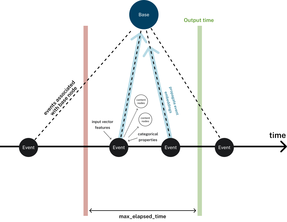
Embeddings computed by FastPath are invariant to absolute timestamps, relying instead on event timings relative to a given observation time of their path. This allows for accurate comparison of paths occurring at different points in time.

Embeddings are computed as a sum of individual event contributions, with more significance assigned to more recent events. Each path is considered independently, which allows for computing embeddings in batches or incrementally, staying compatible with those computed before.

Input

An event sequence consists of a base node with which the embedding will be associated, and one or more event nodes tied to the base node. The input graph may contain an arbitrary number of such event sequences.

There are two supported graph schemas that encode the event sequences.

Event elapsed time

The observation time for an event sequence is given as a property of the base node, or as a parameter applied to all event sequences.

Event times are defined by a property of the event node, or by the node’s position in the event sequence, counted as the number of hops past the first event.

Event elapsed times are then defined as the observation time subtracted by the event time. Only events occurring before the observation time (i.e. with an event time strictly lower than the observation time) will contribute to resulting embeddings.

Event information

An event’s contribution to the resulting embedding depends on the event elapsed time, as well as information tied to the event node. This information can be a combination of three things

categorical properties
relationships to context nodes
floating point feature vectors

Events having both similar elapsed times and similar information will have similar contributions to the resulting embeddings of their respective paths. If either the elapsed time or information differs significantly, their contributions will on average be orthogonal.

What constitutes a significant difference in elapsed time depends on the grid settings and time smoothing.

Syntax

This section covers the syntax used to execute the FastPath algorithm.

Run FastPath.

CALL Neo4j_Graph_Analytics.graph.fastpath(
  'CPU_X64_XS',                    (1)
  {
    ['defaultTablePrefix': '...',] (2)
    'project': {...},              (3)
    'compute': {...},              (4)
    'write':   {...}               (5)
  }
);

1	Compute pool selector.
2	Optional prefix for table references.
3	Project config.
4	Compute config.
5	Write config.

Table 1. Parameters
Name	Type	Default	Optional	Description
computePoolSelector	String	`n/a`	no	The selector for the compute pool on which to run the FastPath job.
configuration	Map	`{}`	no	Configuration for graph project, algorithm compute and result write back.

The configuration map consists of the following three entries.

For more details on below Project configuration, refer to the Project documentation.

Table 2. Project configuration
Name	Type
nodeTables	List of node tables.
relationshipTables	Map of relationship types to relationship tables.

Table 3. Compute configuration
Name	Type	Default	Optional	Description
resultProperty	String	`"embedding"`	Yes	The node property that will be written back to the Snowflake database
baseNodeLabel	String	`n/a`	No	Node label for which output embeddings are desired
eventNodeLabel	String	`n/a`	No	Node label of events related to base nodes
contextNodeLabel	String	`None`	Yes	Node label of context nodes that describe events
eventNodeTimeProperty	String	`None`	Yes	Name of a node property representing time on the event nodes. May be int or float.
nextRelationshipType	String	`None`	Yes	Name of a relationship type between event nodes, indicating order of events
firstRelationshipType	String	`None`	Yes	Name of a relationship type from base nodes to event nodes, indicating the first event for each base node
eventNodeFeatureVectorProperty	String	`None`	Yes	Name of a node property on event nodes which holds numerical features in vector form
eventNodeCategoricalProperties	List of String	`None`	Yes	Names of node properties on event nodes which hold categorical values or lists of categorical values
eventNodeIgnoredCategory	Integer	`-1`	Yes	A category value representing that a category is missing, and is ignored when constructing the event embedding
observationTime	Float	`None`	Yes	The timestamp at which embeddings should be produced. Events at this timestamp or later are not processed.
baseNodeObservationTimeProperty	String	`None`	Yes	Name of a node property on base nodes which holds a number indicating for what timestamp an output embedding should be produced
numTimeAnchors	Integer	`n/a`	No	The number of times in the "grid" . Elapsed time from event to observation time is rounded to this grid. If set to 1, timestamps of events have no effect.
decayRate	Float	`1.0`	Yes	Coefficient controlling the speed of decay of influence of older events
lookbackHorizon	Integer	`n/a`	No	The maximum age of events, relative to the observation time, that are considered for the embedding.
smoothingWindow	Integer	`0`	Yes	Event embeddings are aggregated over a window containing up to 2*smoothingWindow + 1 grid times.
smoothingRate	Float	`0.0`	Yes	Controls how fast expected similarity of events decays as their time-distance increases.
embeddingDimension	Integer	`n/a`	No	The output dimension of the embeddings
randomSeed	Integer	`Random number`	Yes	A random seed which is used for all randomness in computing the embeddings.

For more details on below Write configuration, refer to the Write documentation.

Table 4. Write configuration
Name	Type	Default	Optional	Description
nodeLabel	String	`n/a`	no	Node label in the in-memory graph from which to write a node property.
outputTable	String	`n/a`	no	Table in Snowflake database to which node properties are written.

Configuration concepts explained

This section goes into more detail about how to configure certain aspects of the algorithm.

Graph schema and relationship configuration

The algorithm supports two different schemas for connecting base nodes to event nodes.

To use the first schema configuration you provide a firstRelationshipType and nextRelationshipType, and eventNodeTimeProperty is optional. With this configuration each base and event node is assumed to be part of a path of the pattern: (:baseNodeLabel)-[:firstRelationshipType]-(:eventNodeLabel)-[:nextRelationshipType]-…-[:nextRelationshipType]→(:eventNodeLabel)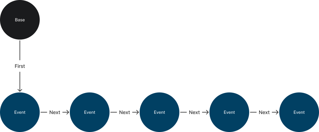
To use the second schema configuration, you provide only a eventNodeTimeProperty. It’s then assumed that each base node has outgoing relationships to each of its event nodes: (:baseNodeLabel)-[:]→(:eventNodeLabel)

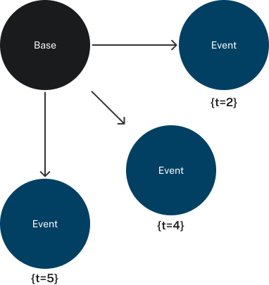
Optionally, the schema can also contain a node label called contextNodeLabel, see Event input below.

Defining event timestamps

There are two ways of specifying timestamps for event nodes. The first way is to provide a eventNodeTimeProperty, in which case each event node must hold a property of that name representing a timestamp.

If however, a nextRelationshipType is provided, eventNodeTimeProperty does not have to be provided. In that case, time stamps are generated in an intuitive way depicted in the picture below.

Timestamp generation

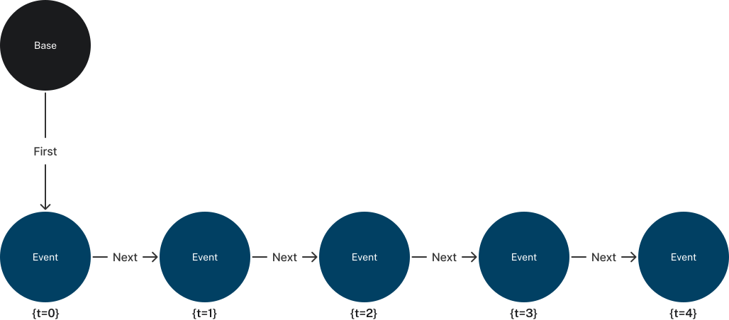
Figure "Timestamp generation": The length of the nextRelationshipType path to an event will define its timestamp. So then the first event node in a base node’s event chain, which is connected via a firstRelationshipType relationship from the base node, will have timestamp 0. The next event node, accessed via a nextRelationshipType relationship from the first event node, will have timestamp 1, and so on.

Please note that you can still provide a eventNodeTimeProperty even if nextRelationshipType is used. In that case, the nextRelationshipType will not be used to infer timestamps, but rather which base node an event node belongs to.

Event input

Information carried by an event can be a combination of three different input sources. The event’s contribution to final embeddings will be a sum of all enabled input sources.

To enable the Context nodes input source you provide a contextNodeLabel. In this case it’s assumed that there may be outgoing relationships from event nodes to context nodes, i.e., the pattern:
(:eventNodeLabel)-[:]→(:contextNodeLabel)
To enable the Event feature vector properties input source you provide eventNodeFeatureVectorProperty. This should be the name of a vector property present on all event nodes.
To enable the Categorical event properties input source you provide eventNodeCategoricalProperties. This should be the name of a property that holds integers representing categories or lists of such integers. The property must be present on all event nodes.

Grid of random vectors

Event contributions to final embeddings are sourced from randomly generated vectors arranged in a grid. The first dimension of this grid is time, containing a number of columns equal to numTimeAnchors, evenly distributed from 0 to lookbackHorizon. Secondly, each categorical event property, each context node, and each position of the event feature space is assigned its own row in the grid.

Each cell in the grid is then assigned a randomly generated vector of size dimension.

An event’s contribution to the final embedding is then an aggregation of vectors from rows matching the event information, and columns in the vicinity of the event elapsed time. How many columns are considered is dependent on the smoothingWindow.

Time smoothing

If smoothingRate is large, only a small amount of smoothing is applied and events that are even a small time apart (enough to be closest to different grid points) will generally have very different embeddings.

If smoothingWindow is 0, the effect is similar to having a large smoothingRate. On the other hand, if smoothingWindow is large in relation to numTimeAnchors, and simultaneously smoothingRate is small, identical events will have similar embeddings even when their timestamps differ a lot.

Output

The output is Snowflake table containing two columns;

nodeid — the node’s id according to an input node table
embedding — the FastPath embedding of the node

The name and location of the table is given in Write configuration.

Example

We assume that we have a Snowflake schema patient_db.general containing the following tables:

patient with columns nodeid and output_time
encounter with columns nodeid, embedding and time
has_encounter with columns sourcenodeid and targetnodeid

These tables represent a graph of medical patient records.

To run the query, there is a required setup of grants for the application, your consumer role and your environment. Please see the Getting started page for more on this.

We also assume that the application name is the default Neo4j_Graph_Analytics. If you chose a different app name during installation, please replace it with that.

The FastPATH algorithm can be run on this graph by executing a statement such as:

CALL Neo4j_Graph_Analytics.graph.fastpath('CPU_X64_M', {
    'defaultTablePrefix': 'patient_db.general',
    'project': {
        'nodeTables': ['patient', 'encounter'],
        'relationshipTables': {
            'has_encounter': {
                'sourceTable': 'patient',
                'targetTable': 'encounter'
            }
        }
    },
    'compute': {
        'baseNodeLabel': 'patient',
        'eventNodeLabel': 'encounter',
        'eventNodeFeatureVectorProperty': 'embedding',
        'baseNodeObservationTimeProperty': 'output_time',
        'eventNodeTimeProperty': 'time',
        'embeddingDimension': 32, -- in reality, a higher value is recommended
        'numTimeAnchors': 30,
        'lookbackHorizon': 3650,
        'smoothingRate': 0.9,
        'smoothingWindow': 2,
        'decayRate': 0.0
    },
    'write': [{
        'nodeLabel': 'patient',
        'outputTable': 'embeddings'
    }]
});

An example of the output is:

JOB_ID	JOB_STATUS	JOB_START	JOB_END	JOB_RESULT
job_91200aa45c0e4b81a14f68a70ecadeda	SUCCESS	2025-11-28T15:35:42.979010	2025-11-28T15:35:58.612925	{ "fastpath": { "predictMillis": 5288 }, "project": { "graphName": "snowgraph", "nodeCount": 11, "nodeLabels": { "ENCOUNTER": { "count": 3, "nodeId": { "dataType": "int8" }, "properties": { "embedding": { "dataType": "ndarray[float32]", "embeddingDimension": 2 }, "time": { "dataType": "int8", "embeddingDimension": 1 } }, "table": "PATIENT_DB.GENERAL.ENCOUNTER" }, "PATIENT": { "count": 8, "nodeId": { "dataType": "int8" }, "properties": { "embedding": { "dataType": "ndarray[float32]", "embeddingDimension": 3 }, "has_diabetes": { "dataType": "int8", "embeddingDimension": 1 }, "output_time": { "dataType": "int8", "embeddingDimension": 1 } }, "table": "PATIENT_DB.GENERAL.PATIENT" } }, "nodeMillis": 563, "relationshipCount": 3, "relationshipMillis": 211, "relationshipTypes": { "HAS_ENCOUNTER": { "count": 3, "direction": "NATURAL", "sourceTable": "PATIENT_DB.GENERAL.PATIENT", "table": "PATIENT_DB.GENERAL.HAS_ENCOUNTER", "targetTable": "PATIENT_DB.GENERAL.ENCOUNTER" } }, "totalMillis": 774 }, "write_node_property_0": { "nodeLabel": "PATIENT", "outputTable": "PATIENT_DB.GENERAL.EMBEDDINGS", "rowsWritten": 8, "writeMillis": 2764 } }

JOB_ID

JOB_STATUS

JOB_START

JOB_END

JOB_RESULT

job_91200aa45c0e4b81a14f68a70ecadeda

SUCCESS

2025-11-28T15:35:42.979010

2025-11-28T15:35:58.612925

{
  "fastpath": {
    "predictMillis": 5288
  },
  "project": {
    "graphName": "snowgraph",
    "nodeCount": 11,
    "nodeLabels": {
      "ENCOUNTER": {
        "count": 3,
        "nodeId": {
          "dataType": "int8"
        },
        "properties": {
          "embedding": {
            "dataType": "ndarray[float32]",
            "embeddingDimension": 2
          },
          "time": {
            "dataType": "int8",
            "embeddingDimension": 1
          }
        },
        "table": "PATIENT_DB.GENERAL.ENCOUNTER"
      },
      "PATIENT": {
        "count": 8,
        "nodeId": {
          "dataType": "int8"
        },
        "properties": {
          "embedding": {
            "dataType": "ndarray[float32]",
            "embeddingDimension": 3
          },
          "has_diabetes": {
            "dataType": "int8",
            "embeddingDimension": 1
          },
          "output_time": {
            "dataType": "int8",
            "embeddingDimension": 1
          }
        },
        "table": "PATIENT_DB.GENERAL.PATIENT"
      }
    },
    "nodeMillis": 563,
    "relationshipCount": 3,
    "relationshipMillis": 211,
    "relationshipTypes": {
      "HAS_ENCOUNTER": {
        "count": 3,
        "direction": "NATURAL",
        "sourceTable": "PATIENT_DB.GENERAL.PATIENT",
        "table": "PATIENT_DB.GENERAL.HAS_ENCOUNTER",
        "targetTable": "PATIENT_DB.GENERAL.ENCOUNTER"
      }
    },
    "totalMillis": 774
  },
  "write_node_property_0": {
    "nodeLabel": "PATIENT",
    "outputTable": "PATIENT_DB.GENERAL.EMBEDDINGS",
    "rowsWritten": 8,
    "writeMillis": 2764
  }
}

The produced node embeddings can be simply explored like so:

SELECT * FROM patient_db.general.embeddings LIMIT 10;

which returns data of the form

NODEID	EMBEDDING
0	    [5.341047,3.848688,-5.973229,-6.814521,4.745209,9.643475,-0.045684,4.210951,-2.004807,4.428759,13.497086,-6.179376,-0.986118,-7.707472,-0.555529,-6.073474,4.083053,1.602635,1.958997,12.649292,-0.603967,10.158164,-0.338394,-0.608493,-4.837356,15.097547,-6.569559,-2.797304,0.338724,6.874722,9.505033,-8.754766]
1	    [-6.724641,-11.390027,-4.453455,4.120544,-2.017518,-2.675358,2.027915,-7.672874,-2.879899,17.374033,11.240053,7.185143,10.593451,-0.032012,6.947659,-29.623604,0.166914,11.507900,-12.466205,-1.891875,-8.164936,7.390674,-10.806652,2.019349,-1.903723,29.574389,1.859032,3.853385,0.566263,-5.038345,4.792415,3.326340]
2	    [-2.920011,-2.048257,-5.708614,-2.373963,-0.244315,2.887959,-23.091557,-0.587305,4.643905,-0.775859,7.227013,-1.861291,-4.952862,-7.039846,-11.932112,-8.986797,-1.304907,2.019032,3.064439,-4.360886,-2.295964,6.218091,0.975781,-3.919339,8.686658,17.961964,-7.780995,-1.146844,-6.269790,20.006420,-1.216949,-3.596368]
3	    [-8.567083,-9.307947,-11.381653,-0.802077,-1.286643,-3.037168,5.494521,-1.814128,-1.623972,-0.085408,-8.678900,6.716533,-3.552778,10.777124,8.609731,2.346340,-6.656413,4.587024,-6.891663,0.081429,-3.976248,-3.998426,-0.445967,4.443917,-7.440049,15.908058,-6.126621,-9.205961,-3.693087,5.798036,-10.521414,25.272419]
4	    [-3.993221,-15.716671,-7.102195,-22.005224,-0.855417,9.282584,-2.253866,-16.234423,24.112732,2.810601,-13.975744,-12.062764,-2.387400,20.061924,-1.067919,12.701017,-4.327281,-17.721920,23.729225,-9.824536,-8.265147,-2.768445,-25.310749,8.047261,13.448681,51.172272,-15.435410,14.756327,-4.342721,11.190716,28.090958,9.425692]
5	    [-13.833055,-3.474358,-29.580704,15.354573,46.242706,13.694808,32.601025,26.757681,-7.090479,57.280357,-0.735581,38.106731,26.968494,3.217232,-23.623219,2.485056,-6.973878,0.877117,-15.995618,55.822735,18.801920,52.809269,-47.148773,39.193768,-4.173650,-12.601570,-14.213085,-21.923597,12.738949,-27.862555,-9.950893,-20.819094]
6	    [13.704840,13.533702,-5.135115,-6.226133,-5.701371,-2.703825,5.956636,3.647114,2.735878,2.559484,-15.129639,9.952298,2.568221,1.664974,-0.048340,-10.921870,-17.725523,1.495797,-9.043520,25.950590,-0.110576,9.694299,-18.446062,-6.852248,6.842557,35.075626,8.634172,7.099162,-5.890983,9.706918,-8.494190,6.583567]
7	    [-2.812654,2.941338,1.067755,-4.293394,-3.086962,-0.469450,3.613479,-2.819084,5.120227,7.050265,-2.466012,-2.169495,0.909174,2.145000,3.638202,-2.498263,-5.502569,-3.852499,5.146134,1.659534,-0.714558,-0.469029,2.176041,-1.869031,-4.940216,3.088835,3.752839,3.714232,-2.807177,-0.698254,-5.012471,2.528090]
8	    [-7.303960,-7.729638,-4.773112,-9.641366,2.609788,-20.279972,6.826665,8.960463,19.718428,3.388449,7.409564,-17.707247,-0.936261,28.070925,-3.749211,-9.148918,16.058552,4.065396,10.297297,9.403608,-10.898782,-10.801480,-25.112486,3.316337,17.157797,12.428331,19.813198,10.889541,-1.723780,-1.651543,-0.261916,9.012156]
9	    [-6.429783,-20.400585,16.191334,-16.042753,9.880158,-5.386495,-10.220762,15.675117,9.438731,-3.742106,10.518373,3.956760,6.789544,-0.625264,-8.893956,1.050145,-15.966327,-6.890019,-2.499497,8.597721,3.010286,3.782031,-10.274326,20.255251,1.046289,17.648533,-6.685064,13.613426,7.041289,13.350776,-3.143279,-5.788550]

Appendix

The following sections provide more detailed information about FastPath for those interested in the inner workings of the algorithm.

How the algorithm works

The below breakdown of the algorithm into steps is conceptual. It does not reflect the actual implementation details such as for example as order of loops, datastructures and more. We will describe how to compute the FastPATH embedding for a base node b which has observation time t_o. The observation time is computed according to one of the chosen parameters observationTime or baseNodeObservationTimeProperty. An arbitrary event which belongs to b will be denoted by e, and its time stamp is assumed to be t_e. At the time t_o, at which we wish to compute the embedding of b, the elapsed time of e is
t_el = t_o - t_e, that is, the amount of time between the timestamp of the event and the observation time of the corresponding base node.

Note, that events may belong to multiple base nodes which have different observation times. This implies that some computations involving an event have to be recomputed for each of its associated base nodes, but luckily these computations are independent of each other.

Preprocess
Pre-process the input into a graph with base nodes, event nodes and optionally context nodes. Base and event nodes are connected and so are events and context nodes. If time stamps are not given for events, time stamps are generated by traversing event chains per base node.
Filter relevant events
Out of the events that belong to the base node b, any event which has elapsed time exceeding lookbackHorizon, or any event which occurred at time t_o or later is removed. The remaining relevant events for b will be called E(b).
Create grid
Create a grid over time subsequently referred to as the grid
Generate random vectors
Sparse random vectors are generated independently per input sources below, if they are selected.
For each time in the grid and input source, generate vectors as follows:
1. Event feature vector properties: a vector r_i,t is generated for each dimension i of the input event feature vectors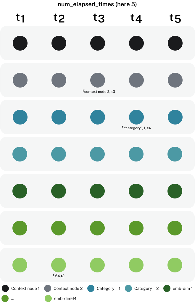
2. Context nodes: for each context node c, generate r_c,t
3. Categorical event properties: for each categorical node property prop and for each value v of that property, initialize a random vector r_prop,v,t.
  If the property value for any event is a list of categories [v₁, v₂, …], and v is any of these values, we initialize a random vector r~prop,v.
Compute event node pre-embeddings
The pre-embedding for an event e at time t is denoted by x_e,t and initialized to all zeros. For all input sources below that apply, weighted sums of random vectors generated in step 3 are added to x_e,t:
1. Event feature vector properties:
  x_e,t += ∑_i r_i,t * inp_i
  where inp is the input vector of e and i ranges over the dimensions of inp.
2. Context nodes:
  x_e,t += ∑_c r_c,t
  where c ranges over all neighbors of the event e.
3. Categorical event properties:
  x_e,t += ∑_prop r_{prop,e.prop,t}
  where prop ranges over all selected categorical event properties.
  Or when e.prop is a list: x_e,t = ∑_prop ∑_{v in e.prop} r_prop,v,t
Compute event embeddings

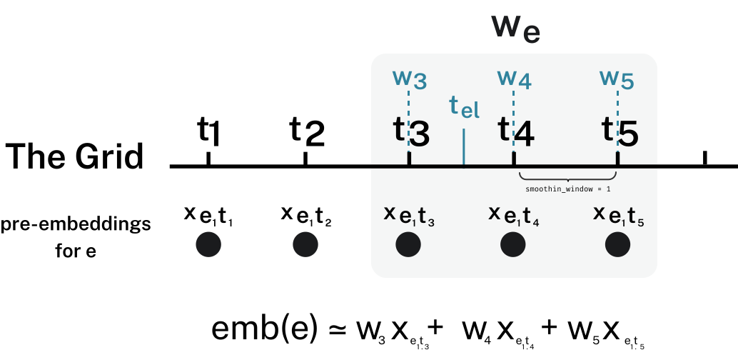
We compute an embedding for e using its earlier derived pre-embeddings at different times. We find the time t_cl in the grid which is the closest to the elapsed time t_el = t_o - t_e. Then adding up to smoothingWindow points in the grid on both sides of t_cl, we to obtain a window W_e of relevant grid times for the event. In the picture, smoothingWindow = 1 and t_cl=t₄. Therefore W_e = {t₃,t₄,t₅}. For each t in W_e we set the weight of the grid point t to be,
w(t) = exp(-|t - t_el| * smoothingRate ) / Z_e,
where Z_e is the constant that ensures ∑_{t in W_e} w(t) = 1.
We can now finally set the embedding of the event at observation time t_o to be
emb(e|t_o) = ∑_{t in W_e} w(t) * x_e,t. We have hence constructed time-smoothed embeddings by taking an average of a grid of pre-embeddings, or basis vectors if you will. The purpose of the time-smoothing mechanism is to ensure that embeddings change continuously with respect to changes in elapsed time, all other factors being equal.
Compute base node embeddings
The embedding for b is finally given by
emb(b) = ∑_{e in E(b)} w_b,e * emb(e)
where
w_b,e = exp(-decayRate * (t_o - t_e)) and E(b) was defined in step 2.

The figure below gives an overview of what influences event embeddings and how they flow to the embedding of a base node, based on the observation time and elapsed times.