How Queries Work in Neo4j

About this module

At the end of this module, you will be able to:

Describe the components of query processing.
Describe an execution plan.
Describe the cost of accessing nodes, labels, properties, and relationships
Understand the graph you will be working with:
- Data Model
- Indexes and Constraints
- DB Stats

Components of a query

When you execute a Cypher statement that is a query against the graph, the following resources are used:

If the query is not already in the Execution Plan Cache, the query is compiled into an execution plan in the Neo4j DBMS.
The execution plan executes in the Neo4j DBMS to retrieve data. The Page Cache is used to hold the data in memory. Heap memory is also used to hold intermediate execution data used for aggregating, sorting, and path building.
Neo4j DBMS returns results to the client.

Each of these steps takes time and your goal is to minimize these times.

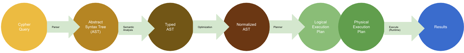
Query processing steps

Here is a little more detail about how a query is processed.

The query is tokenized and then parsed into an Abstract Syntax Tree (AST).
Semantic checking is done on the AST to make sure that variable types and scopes are valid. Otherwise an error is returned to the client.
The AST is optimized so that some syntax is normalized. Examples of this are:
1. Move labels from the MATCH clause to the WHERE clause.
2. Supressing redundant WITH clauses.
3. Expanding aliases such as RETURN * becomes RETURN x AS x, y AS y.
4. Folding constants such as 1 + 2 * 4 becomes 9.
5. plus many more optimizations…
The Normalized AST is used to create a query graph that is used to create the logical execution plan. The planner then uses its knowledge of the graph metadata to produce the physical execution plan which is an optimized version of the logical execution plan.
The physical execution plan runs in the appropriate runtime, which is based upon the operations in the execution plan. Some operations cannot run in parallel so this affects which runtime is used to execute the query. And finally the runtime returns the results to the client.

Query performance factors

There are other factors that affect the performance of a query:

Version of Cypher you are using.
Cypher runtime you are using. Note that the runtime used may depend on the operations used for a query.
Cypher replanning settings.

These are described in the Query Tuning Documentation.

How query execution plans are created by the query planner is very much dependent on the version of Neo4j you are using. That is, you must re-measure your query performance and possibly change queries with each version of Neo4j.

For this course, we use Neo4j Desktop which supports Neo4j Enterprise for development. We are using Neo4j 4.1 for all query executions.

Execution Plan Cache

The Execution Plan Cache is an in-memory data structure that keeps track of query strings and their associated execution plans that have been executed against the DBMS.

Each execution plan is cached by the query string as well as the types of parameters.
- The query string is case-sensitive:
  - Example: MATCH (a:Actor) is different from MATCH(A:Actor).
- Literal values are part of the query that is cached:
  - Example: MATCH (a:Actor {name: 'Joe'}) is different from MATCH (a:Actor {name: 'Alice'}).
Best Practice: Always use parameters for literal values in your queries.
- Example: MATCH (a:Actor {name: $actorName})
- Parameter types are used to create the optimal execution plan.
  - A parameter mapped as type String can be used for index-backed ORDER BY.
If the graph has changed significantly, an execution plan could become stale because the prerequisites for the planning have changed. In this case, the execution plan is removed from the Execution Plan Cache.
If the Execution Plan Cache is full, Neo4j removes a least recently used query to make room for a different query. This behavior is configurable with cypher.statistics_divergence_threshold.

Execution plan

The compilation of the Cypher query results in the execution plan. The execution plan is shown using the EXPLAIN or PROFILE clauses in a Cypher query. The execution plan is a tree structure of steps (operators) that execute, some in sequence and some in parallel, depending on the steps. A leaf step is typically the beginning (anchor) of the query. A step in the execution plan takes zero or more "rows" of data to produce "rows" of data that are passed to the next step in the execution plan.

When you specify EXPLAIN, the query does not execute, but it returns the execution plan with the estimated rows.

Execution plan - PROFILE

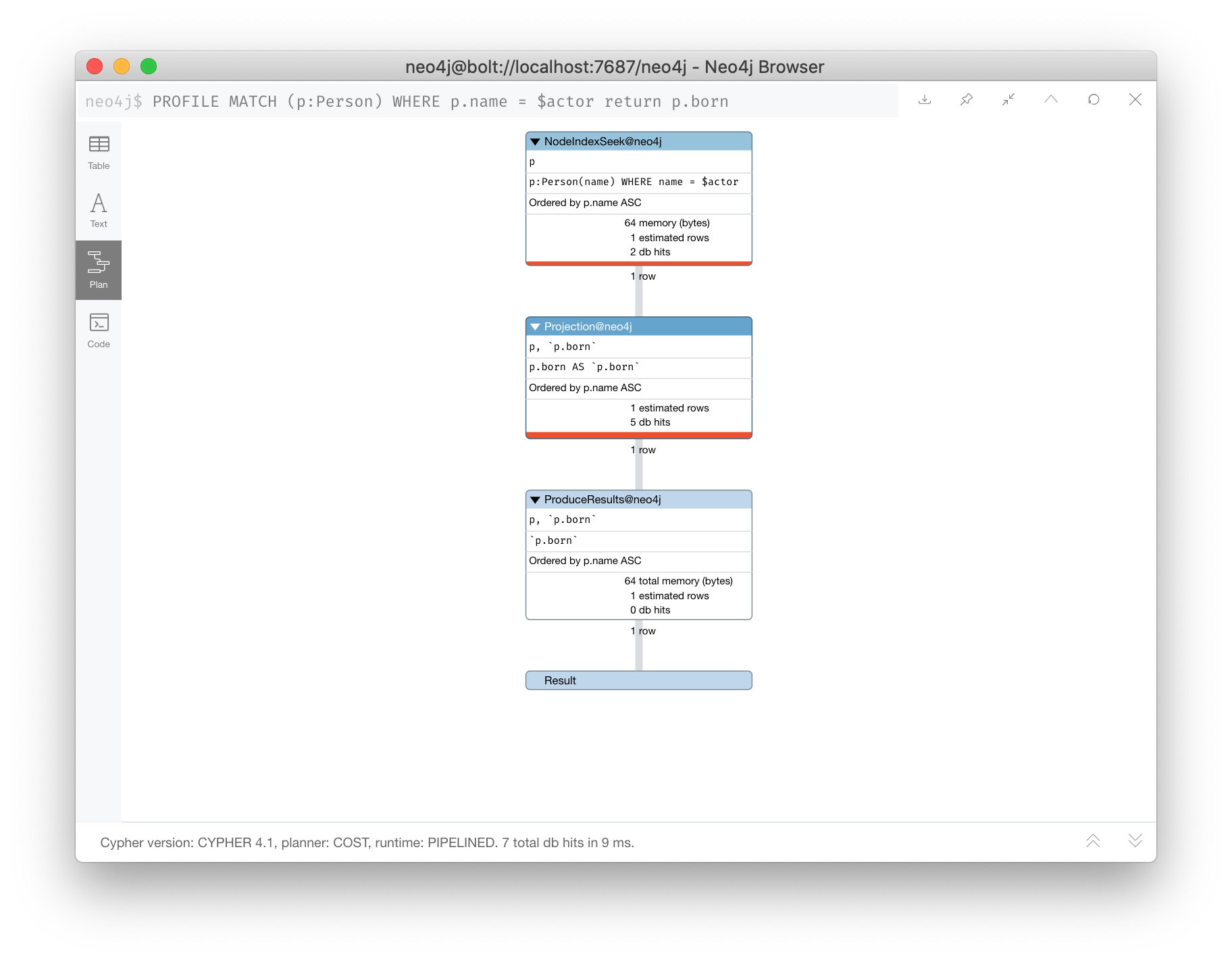
The query executes when you specify PROFILE and includes these values:

rows: This is probably the most important metric you will aim to reduce in a query. The rows passed from one step of a query to the next require both memory and CPU resources. What you want to watch for are spikes in the number of rows passed between steps as these may be areas where you can tune.
db hits: You can think of a db hit as an abstract unit of work. Db hits from one step to another cannot really be compared due to the complexity of how data is stored physically. You may not always be able to reduce the number of db hits. You also want to reduce the amount of data that needs to be retrieved from the graph. If you can confine retrievals to what is in indexes, the less data needs to be retrieved from the graph.
elapsed time: Elapsed time includes the time to run the query as well as return results. Whether data needs to cross a network may also impact the elapsed time.
memory: The amount of extra heap required to execute that operator in the execution plan.

Page Cache

The Page Cache is an in-memory copy of part or all of the graph. The area of memory used for Page Cache is managed by the DBMS, meaning that it is not automatically garbage collected in the JVM. Ideally, you want as much of the graph to be in memory as possible (Hit Ratio), but this will depend upon the size of the graph and the amount of RAM on the system where the Neo4j instance is running. Later in this course, you will see how the page cache is used in the steps of an execution plan when it executes.

You use the :sysinfo Neo4j Browser command to examine the usage of the Page Cache:

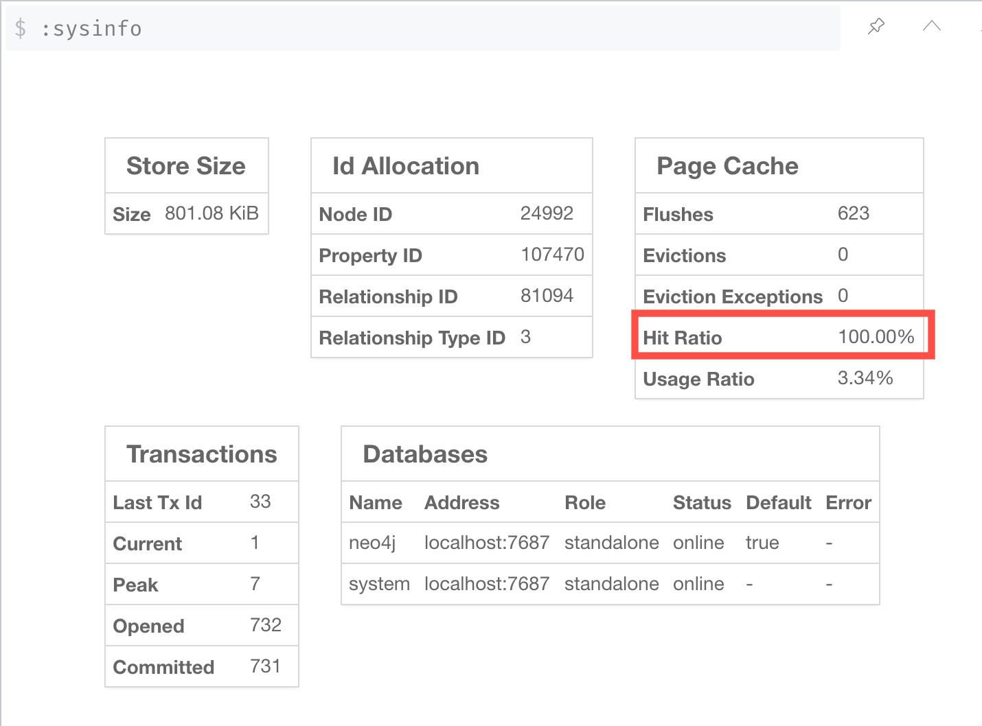
Ideally, you want the utilization of the Page Cache to be as close to 100% as possible. If you see that in your application, there are a lot of flushes of the Page Cache, then you must consider, if possible, adding more RAM to the system.

Heap memory

Heap memory is used in all steps of query processing and is managed by the Java Runtime, not by the DBMS. That is, it is subject to garbage collection in the JVM. The creation of the objects, for example AST, used to parse, optimize, and collection intermediate results is all allocated in the heap. You can help to ensure that heap memory does not suffer from unwanted garbage collection by configuring a heap size that is the size of RAM minus the Page Cache size (for small systems, you can choose heap sizes of 8G, 16G, or 28G).

Result set

The result of a query is returned to the client with the RETURN clause. In many cases the data is sent over a network so minimizing the amount of data that needs to be read from the database, formatted and sent back to the client will be a goal.

Understanding execution plans

The most important task for you as a developer is to understand what an execution plan is, how to interpret it, and most importantly, how to make it performant. To understand the execution plan, you must understand how a query starts and then how it is processed as the nodes are traversed in the graph.

Next, you will learn about:

Anchoring
Expansion
Eager operators
Query runtimes
Goals for improving query performance

You can read the details of execution plans here.

Anchor of a query

When the execution plan is created, it determines the set of nodes that will be the starting points for the query. The anchor for a query is often based upon a MATCH clause. The anchor is typically determined by meta-data that is stored in the graph or a filter that is provided inline or in a WHERE clause. This meta-data is the count store that you will learn about later in this lesson. The anchor for a query will be based upon the fewest number of nodes that need to be retrieved into memory.

Here are three simple queries for a graph that has 6231 Movie nodes and 18,776 Person nodes:

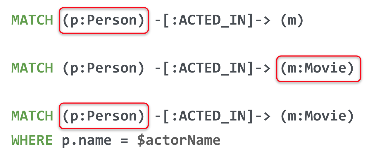
In the first statement, the Person nodes will be the anchor for the query. This is because there are a total of 24,993 nodes in the graph which is what m represents. There are only 18,776 Person nodes so the execution will retrieve fewer nodes if it anchors with the Person nodes.

In the second statement the Movie nodes will be the anchor for the query because there are fewer Movie nodes than Person nodes.

In the third statement, a filter is specified which reduces the number of nodes that will be retrieved for the Person node satisfying the filter is the anchor for the query. If the Person nodes has an index on name, it only retrieves one record. If there is no index, it needs to scan/filter all Person nodes for the name property.

Multiple anchors

By default, an anchor set of nodes is determined by the metadata related to the query path and WHERE clauses to filter the query. In some cases you may have more than one set of anchor nodes.

For example, you can specify:

MATCH (p1:Person)-[:ACTED_IN]->(m)
MATCH (n)<-[:ACTED_IN]-(p2:Person)
WHERE p1.name = $actor1
  AND p2.name = $actor2
  AND m=n
RETURN m.title

In this example, all p1 nodes are retrieved as well as all p2 nodes. This query has two sets of anchor nodes. It retrieves the anchor nodes before the equality filter is applied. The query planner tries to apply filters as early as possible to reduce cardinality (number of rows).

Expand to follow paths

After the anchor nodes have been retrieved, the next step if the query specifies a path is to follow the path. The loaded, initial nodes that are part of the anchor set have pointers to relationships that point to nodes on the other end of the relationships.

The goal here is to eliminate paths from the nodes in memory to nodes that will need to be retrieved. This is where specificity in the relationship types is important in your data model.

For example:

MATCH (m:Movie)<-[:DIRECTED]-(p:Person)
WHERE p.name = $name
RETURN  m.title

This query will expand to fewer Movie nodes than this next statement which retrieves Movie nodes with both the ACTED_IN and DIRECTED relationships:

MATCH (m:Movie)<--(p:Person)
WHERE p.name = $name
RETURN  m.title

In addition, the expansion may lead to the need to inspect properties of the relationship and/or the properties of the Movie node. This inspection means that the nodes are brought into memory and possibly eliminated from the nodes in memory after they have been retrieved.

Cypher queries with multiple MATCH statements may execute differently than what you may expect. This is covered in a later lesson of this course.

Example 1: A simple execution plan

Here is a simple example rendered in Neo4j Browser where we use PROFILE to display the execution plan and execute the query:

PROFILE MATCH (m:Movie)<-[:DIRECTED]-(p:Person)
WHERE p.name = $name
RETURN  m.title

Here is the execution plan:

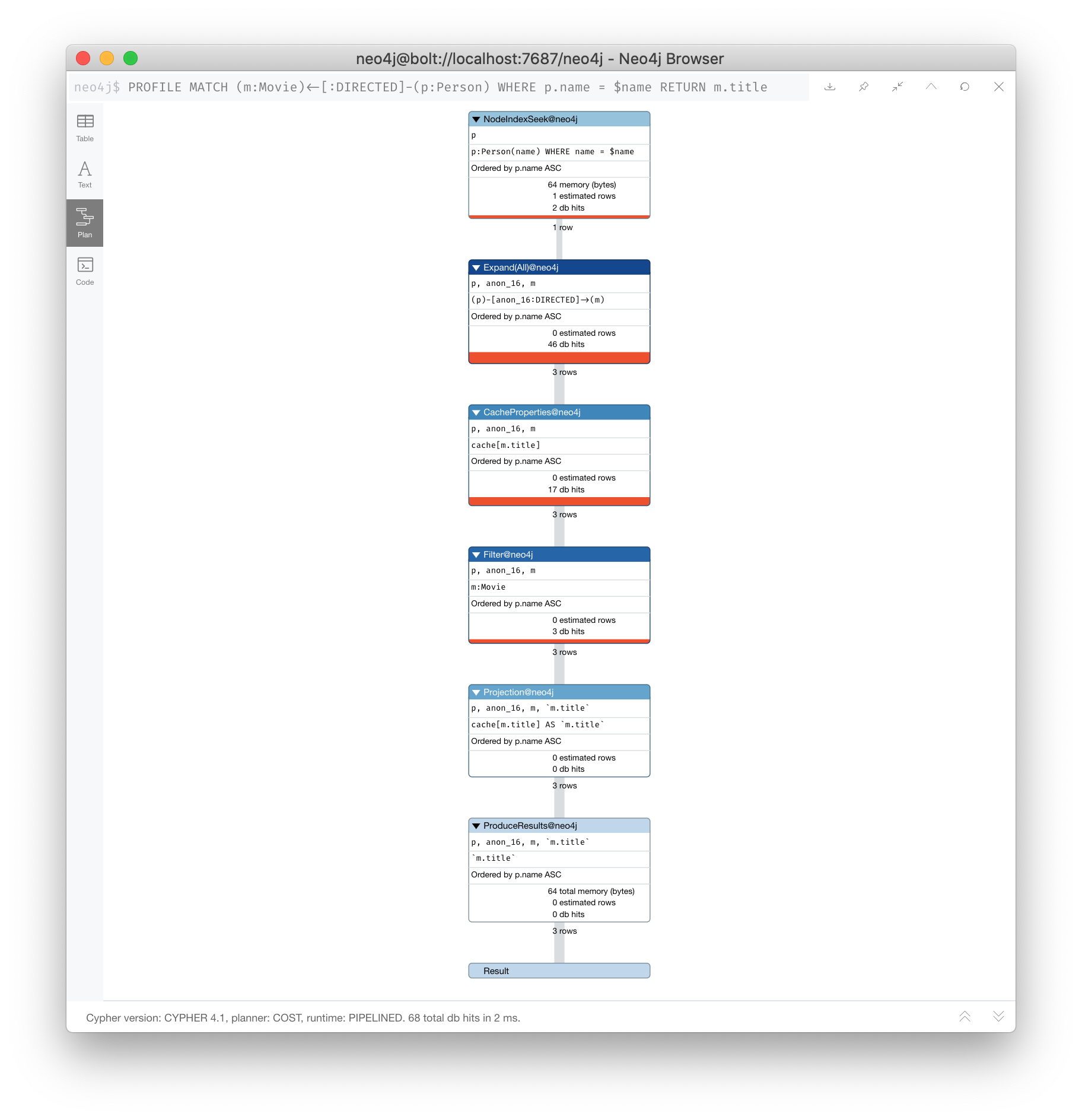
The first step is the NodeIndexSeek operator. This is the operator used to anchor the starting point in the query. This first step takes no rows as input, but produces one row based upon the value specified in the WHERE clause. Because our graph has an index on that property, the index is used. You want all of your query anchor steps to use an index if possible. Note that the index is only used to find the anchor set of nodes and is not at all used for traversing the graph. If the index represents a unique constraint, then only one node is retrieved.

The next operator in the execution plan is Expand(All). This operator traverses all DIRECTED relationships from the single Person node retrieved in the first step and returns three rows where the first element in each row is the Person node and the second element in the row is the Movie node that is on the other end of the relationship traversed.

The next step in the execution plan is CacheProperties. In this step, if any nodes in the rows have properties stored with the nodes, those properties may be cached in memory. In this case the title property of the Movie node is cached, as well as the name property of the Person node.

The next operator, Filter is used to finalize the rows that have been passed in from the previous step to ensure that all predicates for filtering are true. In this case it checks for the Movie label on the nodes and all 3 rows are passed to the next step.

The next operator, Projection is where the results are prepared to be returned to the client. In this example, the rows that contain the Person and Movie nodes are transformed to rows that contain only the title property as that is the property specified in the RETURN clause.

And the final operator, ProduceResults prepares to send the results back to the client. In this query, it will be three rows, each containing the title of a Movie node.

Notice also that steps that incur db hits are highlighted in orange. Observing db hits is important as it may show areas of the query that could be improved.

Another visual advantage for viewing execution plans in Neo4j Browser is that the thickness of the arrows between steps is proportional to the number of rows being passed to the next operation.

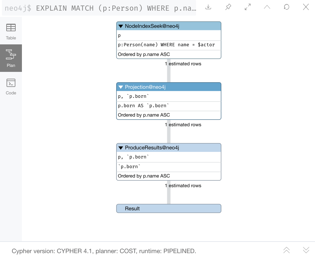
Example 1: A simple execution plan (cypher-shell)

You can also examine the execution plan in cypher-shell:

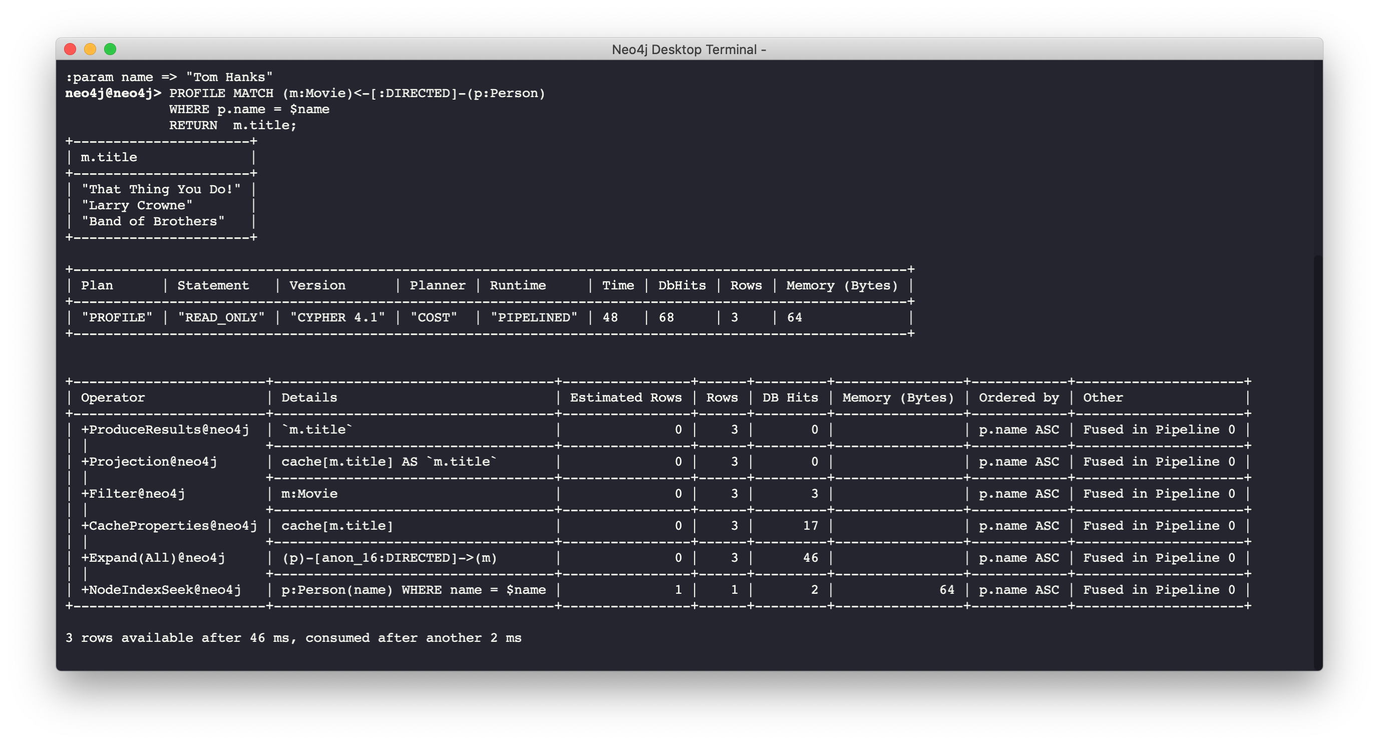
When interpreting the execution plan in cypher-shell, you begin at the bottom and move to the top, but you can see that it shows the same information as what you see in Neo4j Browser.

Example 2: A more complex execution plan

Here is another execution plan to illustrate how it is executed. Here is the Cypher code where the graph contains Movie nodes with a genres property, but no Genere nodes. This code extracts the genre information from the Movie nodes, creates the Genre nodes and the :IS_GENRE relationships between Movie nodes and Genre nodes.

PROFILE MATCH (m:Movie)
UNWIND m.genres AS name
WITH  name, collect(m) AS movies
MERGE (g:Genre {name:name})
WITH g, movies
UNWIND movies AS m
WITH g,m
MERGE (g)<-[:IS_GENRE]-(m)

For most execution plans, you will want to view them in full-screen mode and possibly zoom out.

Here is the execution plan:

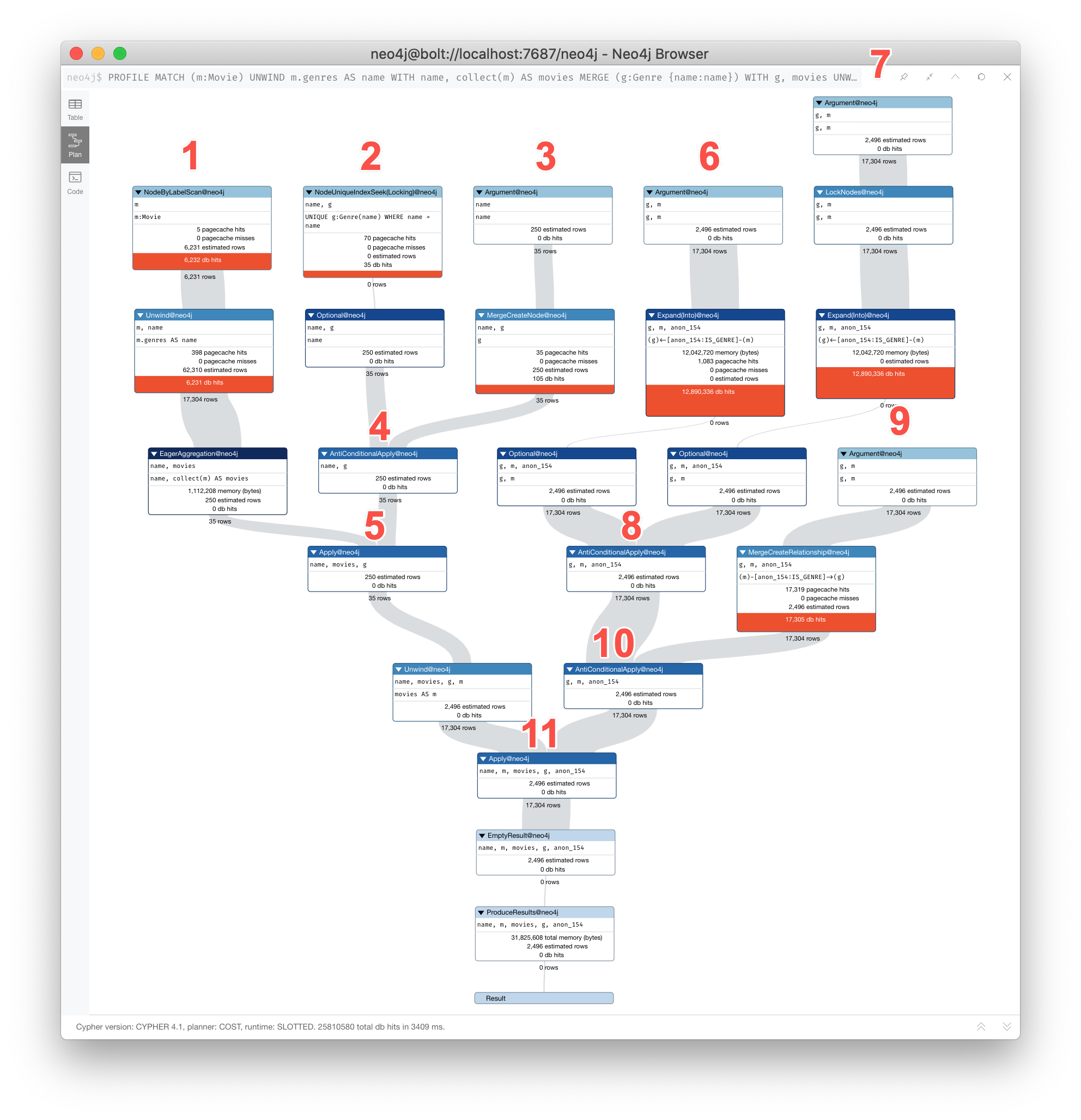
This query is a little different because it is modifying the graph, but the point of this example is to illustrate how the execution plan works. It first executes the three operations under (1). It cannot execute (5), until the operations execute under (1) and (4). It cannot execute (4) until all of the operations under (2) and (3) execute, etc.

Example 2: A more complex execution plan (cypher shell)

Viewing a complex execution plan is sometimes easier in cypher-shell because the steps are presented in tabular format.

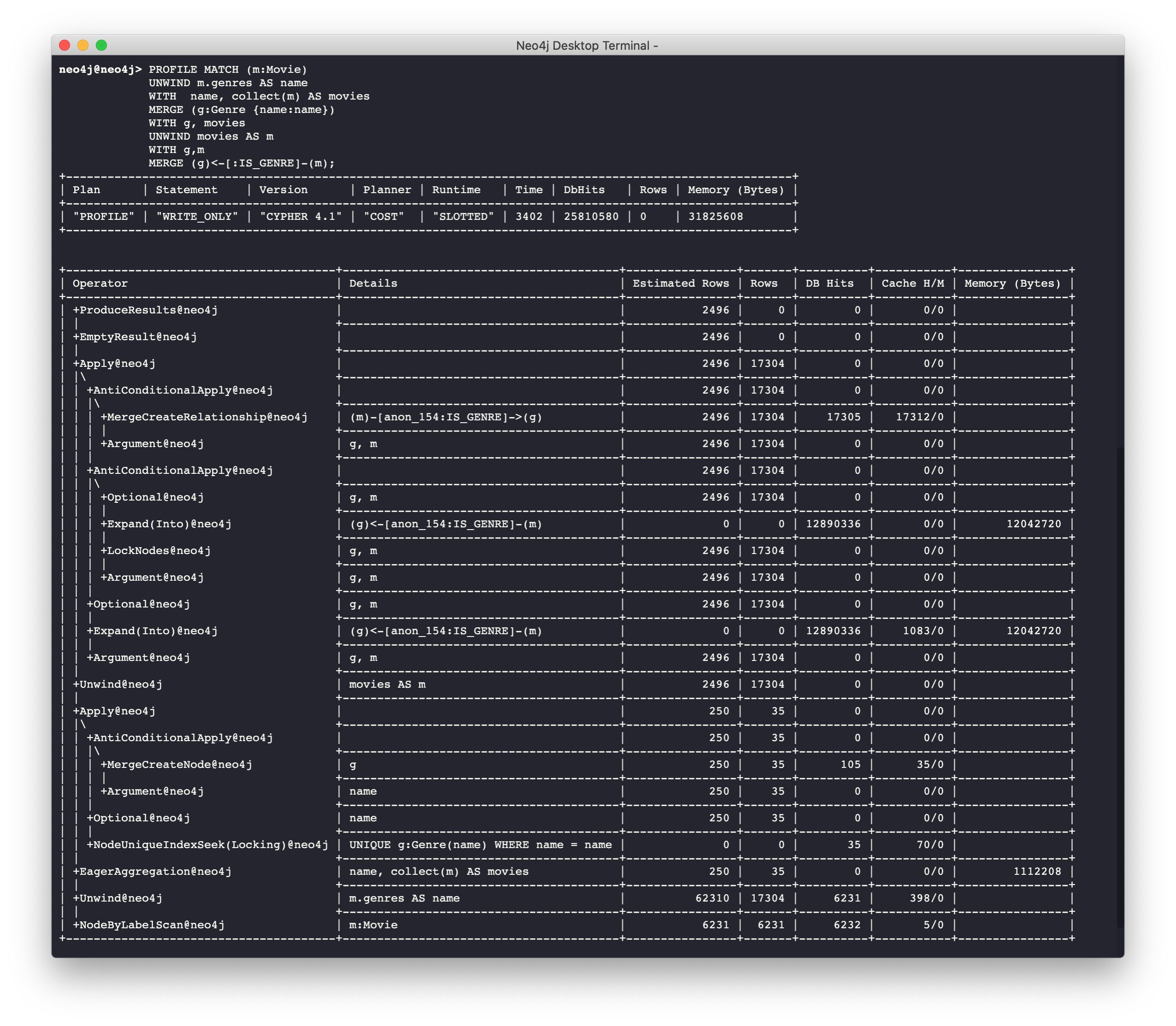
For a more complex execution plan, there are parts of the plan where all steps must execute at a given level before you go to the next step. For example, all steps under the first AntiConditionalApply which are Argument and MergeCreateNode must execute first before the AntiConditionbalApply step executes.

You can use either Neo4j Browser or cypher-shell for your query tuning analyses. Some things render better in cypher-shell while others can only be easily viewed in Neo4j Browser.

During this course, you will see some of the most commonly used operators in an execution plan. These operators are described here in the documentation.

No Eager operations

The execution plan will execute steps of the query on sets of data (rows) retrieved from the graph.

Here is the order that operations execute when the query contains no eager operators or Cypher that requires eager operations:

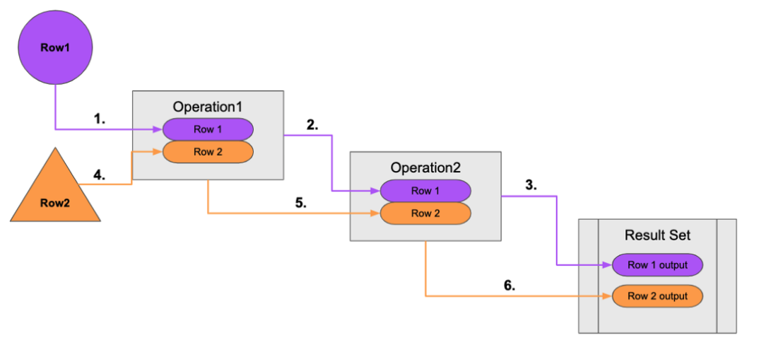
A row is retrieved, then the next operator uses that row, and so on until the result is produced. Then the next row is retrieved and processed.

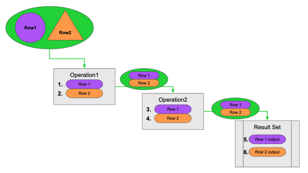
Eager operations

Eager operations require that all rows are retrieved and operations are performed on all rows until the result is produced. Eager operations are explicitly used when the Cypher code includes keywords or functions that require eager behavior during the query processing. Eager operations are implicitly used in execution plans to prevent infinite loops.

Here is the order that operations execute when the query includes implicit or explicit eager operators:

Example: Implicit eager operations enforced by the query planner

Here is an example where the execution plan is created operate "eagerly" to prevent infinite processing.

MATCH (p:Person)
CREATE (p2:Person {name:p.name})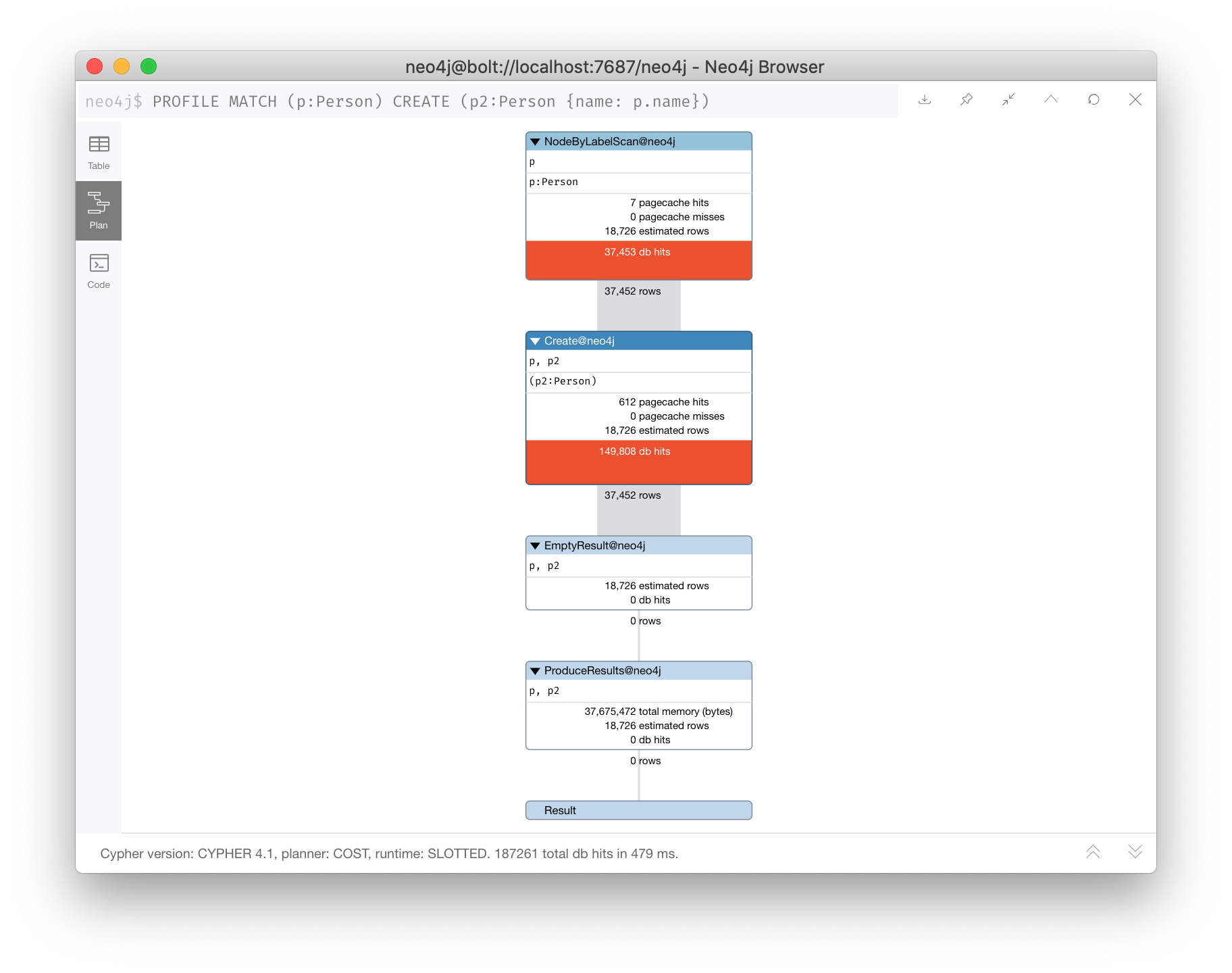

When this query executes, all existing Person nodes are retrieved as rows and then Person nodes are created that has the same name as each Person row previously retrieved. If the query planner had not interpreted this sequence of Cypher clauses this way, there would have been an infinite number of Person nodes created because newly-created ones would continue to be retrieved with the initial MATCH clause. Sometimes the query planner forces eager operations, just to be safe.

Example: Explicit eager operations with a `FOREACH`

Here is another example. A FOREACH clause requires that all rows have been retrieved before it processes the rows used in the FOREACH clause.

PROFILE
MATCH p = (a:Actor)-[:ACTED_IN]-(m:Movie)
WHERE 1942 <= m.releaseYear <= 1945
FOREACH (x IN nodes(p) | SET x.USWarTime = true)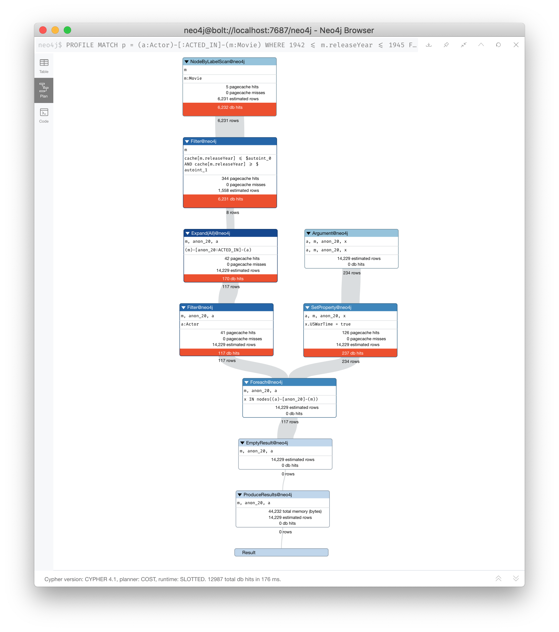

When this query executes, all nodes in the pattern must be retrieved with Expand(All) before the USWarTime property is set for all of the nodes in the path in the FOREACH clause. Notice that in this execution plan the Expand(All) step is in dark blue to call it out as an operation that is eager. The expansion must be done before the next query steps occur.

Eager aggregation

Eager aggregation is also enforced in an execution plan. The aggregating clause or function requires that all nodes or property values are retrieved so that the aggregation can be completed.

These functions and clauses will force the execution plan to complete processing for all rows before continuing with the rest of the query:

ORDER BY (if not using an index)
DISTINCT (for row selection)
aggregating functions such as collect(), count(), avg(), min(), max() etc.

You will learn about aggregation and how it can be controlled for tune your queries in the next lesson.

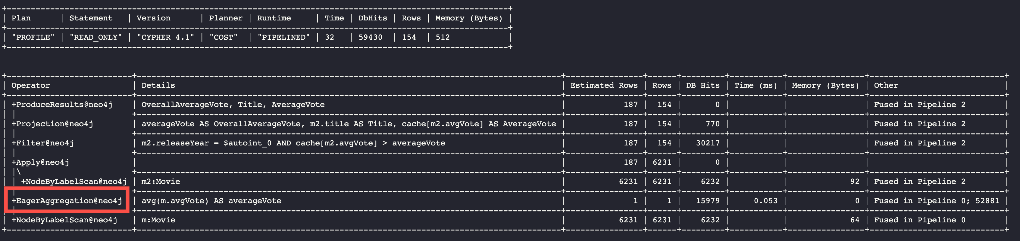
Example: Eager aggregation

Here is an example of eager aggregation in an execution plan where the call to avg() requires that all movie nodes are retrieved before the next step in the execution plan.

PROFILE
MATCH (m:Movie)
WITH avg(m.avgVote) as averageVote
MATCH (m2:Movie)
WHERE m2.releaseYear = 2010 AND m2.avgVote > averageVote
RETURN  averageVote AS OverallAverageVote, m2.title as Title , m2.avgVote as AverageVote

Here is the execution plan in Neo4j Browser:

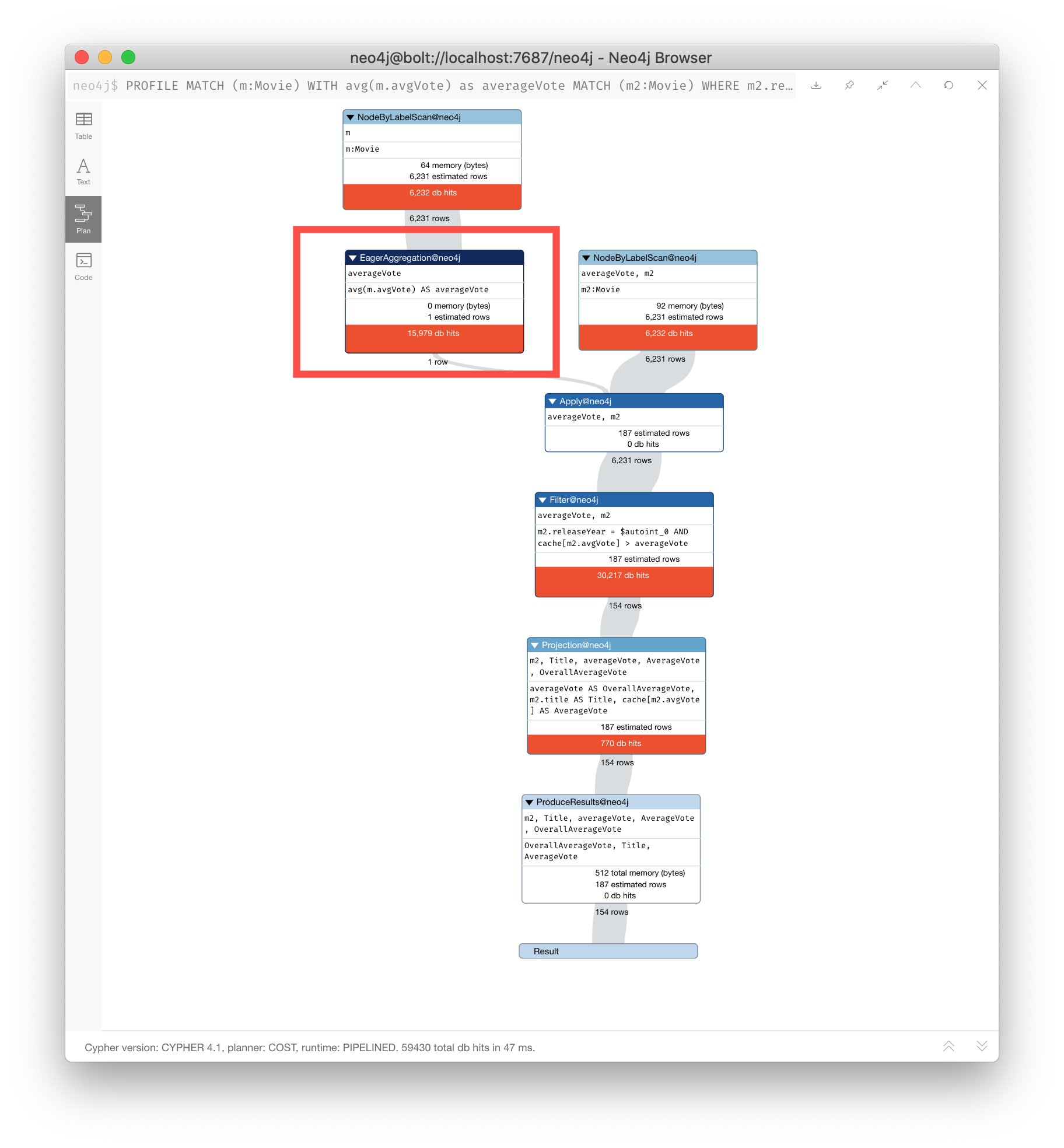
Any eager operator is shown in dark blue to call it out.

Example: Eager aggregation (cypher-shell)

And here is the same execution plan in cypher-shell:

SLOTTED vs. PIPELINED operators

In Neo4j 4.1, many performance improvements have been made to the Cypher runtime by implementing the PIPELINED runtime for many operators. Most read-only operators use PIPELINED runtime by default, but there are some that still use SLOTTED. Which runtime used by each operator is in the Cypher Reference Manual. Operators that modify the graph use SLOTTED runtime which is slower.

Part of your query tuning exercise is to identify queries that do not use PIPELINED.

SLOTTED and PIPELINED are supported in Enterprise Edition. If you are using Community Edition, you must use Interpreted.

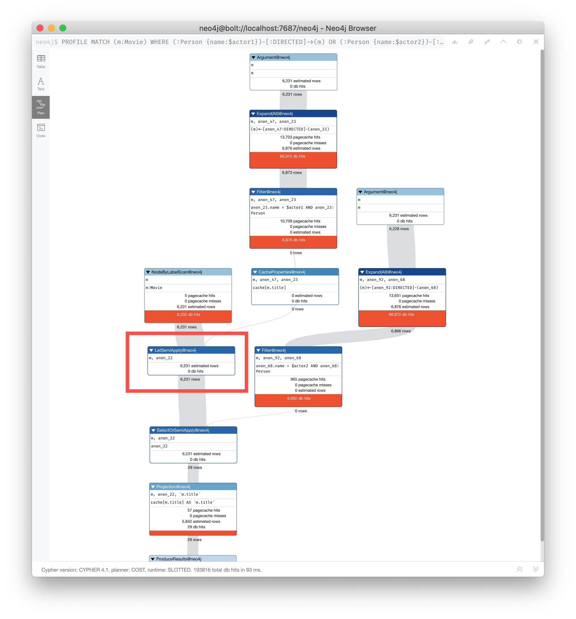
Here is an example where we want to return the titles of the movies directed by two people. $actor1 is 'Tom Hanks' and $actor2 is 'Clint Eastwood':

PROFILE
MATCH (m:Movie)
WHERE (:Person {name:$actor1})-[:DIRECTED]->(m)
OR (:Person {name:$actor2})-[:DIRECTED]->(m)
RETURN m.title

Here is the execution plan, where we see that SLOTTED is used because we require the LetSemiApply operator:

Rewrite query to use PIPELINED

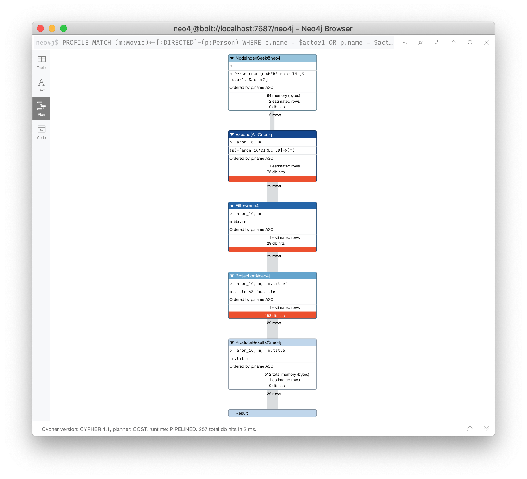
Strive to eliminate SLOTTED from your (read-only) execution plans by rewriting the query to not use operators that must use SLOTTED. For example, this query can be rewritten to:

PROFILE
MATCH (m:Movie)<-[:DIRECTED]-(p:Person)
WHERE p.name = $actor1 OR p.name = $actor2
RETURN m.title

This has a much better execution plan:

Goals for improving execution plans

As you gain experience with query tuning and viewing execution plans, your goals are:

Avoid redundant work and operations.
Early in the query, eliminate data that is going to be filtered out later in the execution.
Recognize less expensive ways to do what you want:
- Improve the Cypher statement.
- Can you ensure query is using PIPELINED?
- Will APOC perform better for some processing?
- Will a stored procedure perform better?

In this course we do not cover writing Cypher queries using APOC or writing custom store procedures.

Information used during query processing

Node labels provide a way to group nodes to make the query more specific. Neo4j automatically creates indexes for faster access to node in a group.
Node degree is a count of the relationships to or from a node. The degree of a node is used to determine if it is a good anchor starting point for traversal, especially if one end of the pattern’s nodes have a higher degree.
Count store contains metrics about the labels and node degrees that can be used to estimate which plan is the best at runtime. You will learn more about the count store later in this lesson.
Indexes are used only for the initial anchoring of the query (beginning MATCH pattern). You can use one or more indexes to anchor the query, but by default only one index is used.
Relationships are traversed to discover and collect nodes that satisfy all or part of the query.
Properties are initially accessed to filter a query or refine the number of rows processed in the execution plan. Some properties are in the same physical location as the node or relationship, but there is no guarantee of this proximity. Properties are also used to collect information during the retrieval, or to collect information to return to the client.

Hierarchy of accessibility

For each data object, how much work must Neo4j do to retrieve the data?

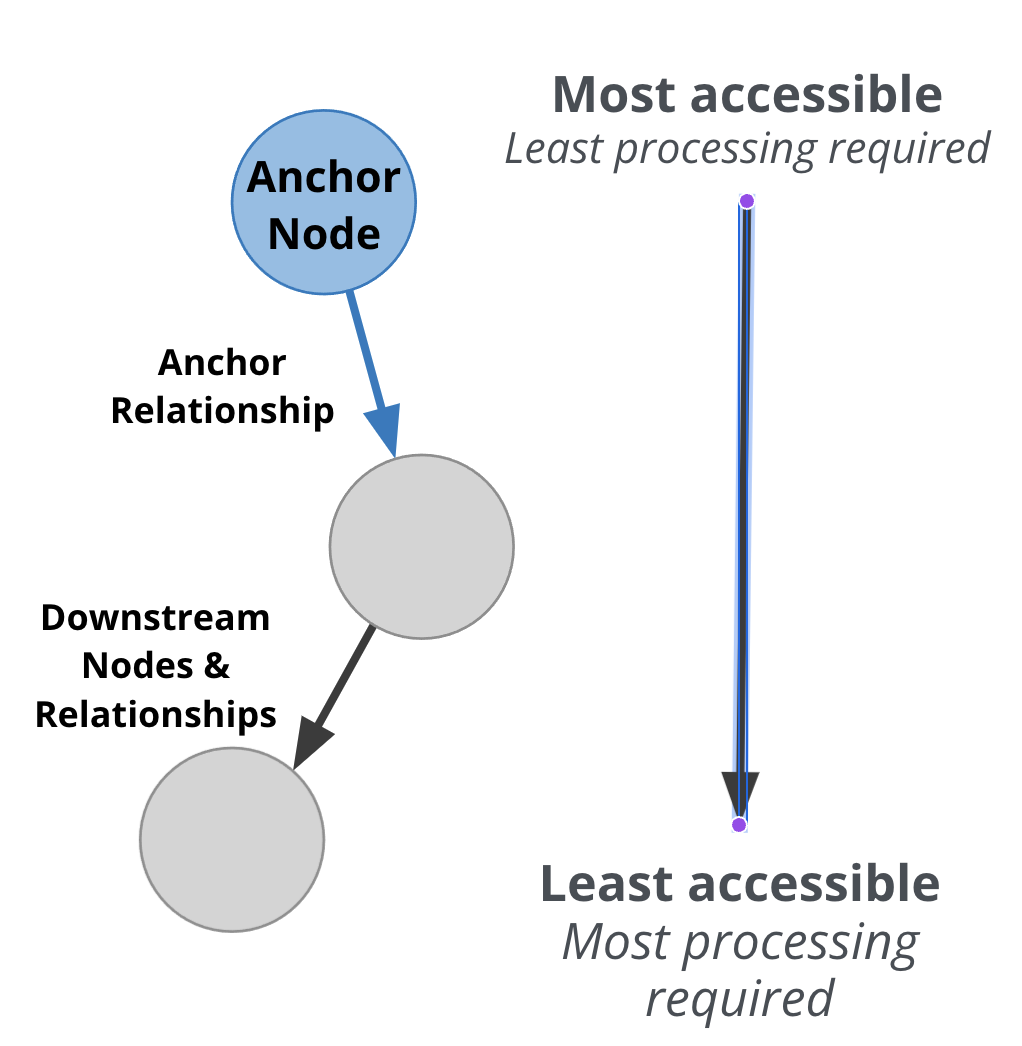
Here is the cost of access from least expensive to most expensive:

Anchor node label, indexed anchor node properties, indexed anchor relationship properties
Non-anchor relationship types and direction
Non-anchor node labels
Non-anchor properties

When analyzing queries, you must always remember how expensive nodes, relationships, and properties are to access.

Starting in Neo4j 4.3, you can define indexes on relationship properties and in Neo4j 4.3 Enterprise Edition, you can create constraints on relationship properties.

Understanding the graph you are working with

To understand the work that is required to execute a query, you must know:

The data model for the graph.
What indexes exist in the graph.
DB Stats for the graph.

Data model for the graph

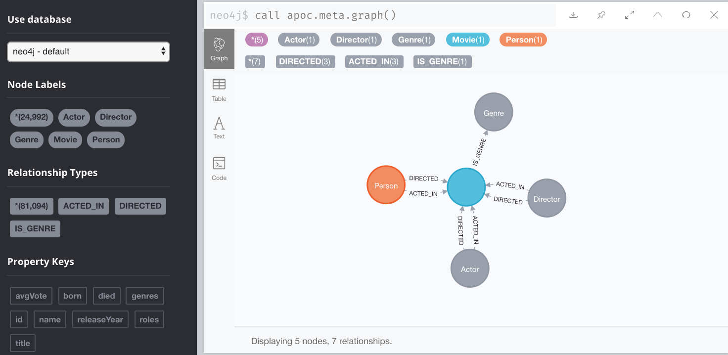
The APOC library contains many useful procedures that will help you with your database. One of the procedures is to retrieve high-level meta-data from the graph.

To inspect how nodes and relationships are used in the graph you simply execute:

CALL apoc.meta.graph()

This is obviously best viewed in Neo4j Browser.

If you view the data for each node presented, it will also display counts for each node and relationship type.

Indexes and Constraints

Part of understanding the performance of Cypher queries is to know what indexes are in the graph that are used during query execution. You learned that node labels are automatically indexed in the graph so the graph engine has efficient access to nodes of a particular type. You must understand what indexes exist for the properties in the graph. The index is only used for determining the anchor nodes for a query (MATCH/WHERE) clauses.

As a starting point, query the graph to learn about all of the indexes defined:

:schema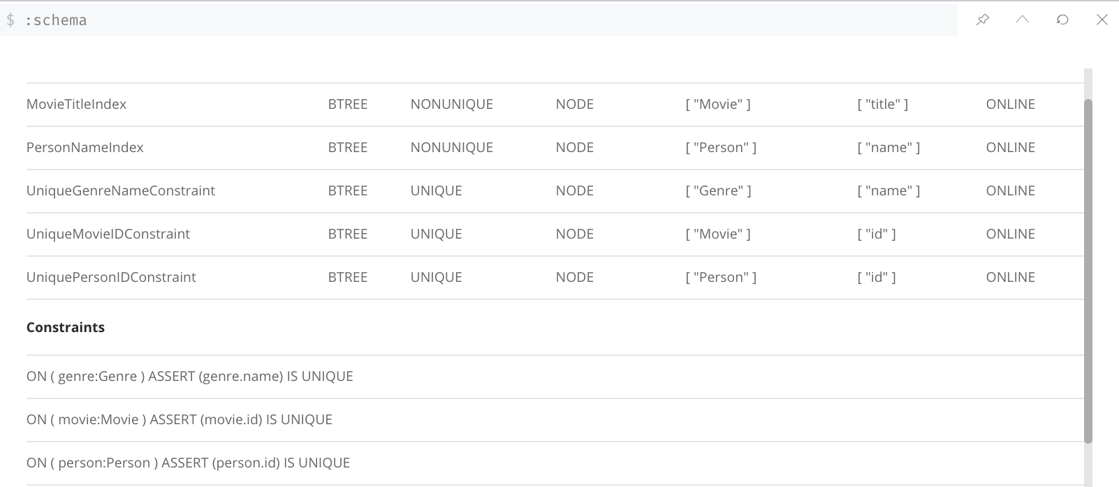

Here we see that in this graph, a unique index exists for the Genre.name property and indexes exist for the Movie.title and Person.name properties. Having these indexes will make anchoring a query much faster.

DB Stats for the graph

You can certainly perform Cypher queries to retrieve information about the number of nodes or relationships of each type, but the easiest way to learn about this meta-data is by retrieving the count store data. You can retrieve count store information with this statement:

CALL apoc.meta.stats()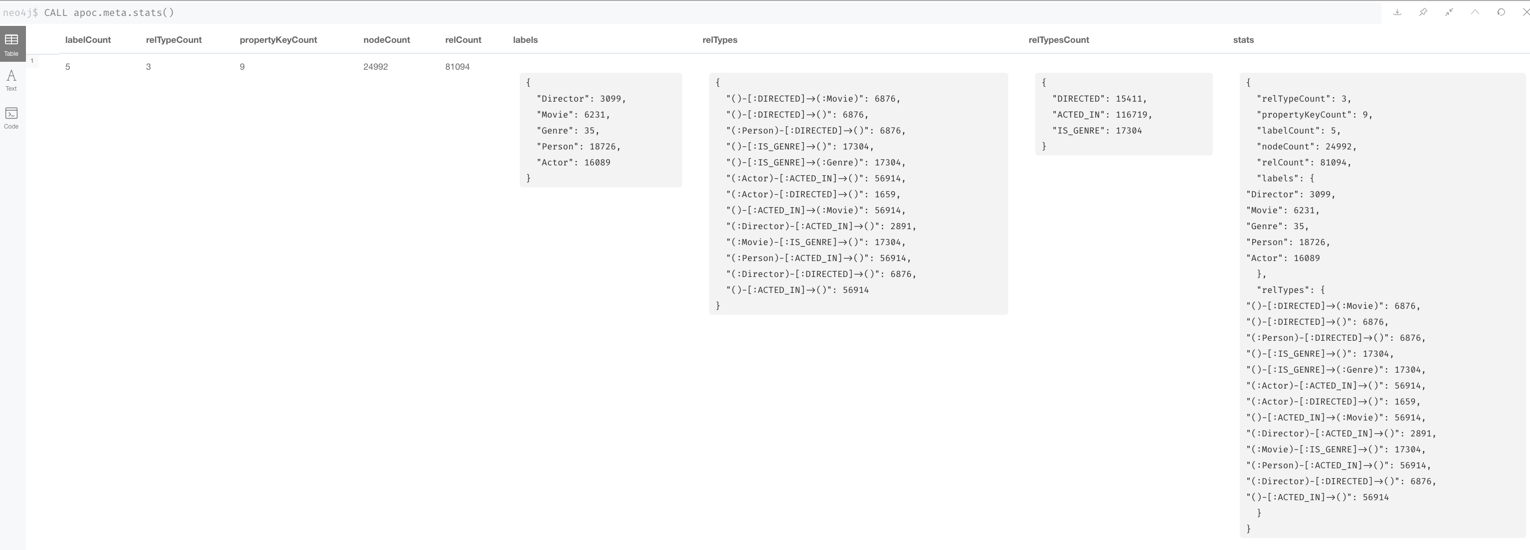

This procedure returns very useful information, all of which is used to create the execution plan for a query.

Count store

The count store is transactionally updated as nodes and relationships are added to the graph. The meta-data in the count store is used to determine whether it is faster to use an index or the count. Another type of information that is kept in the count store is the number of nodes a particular index value points to (called index selectivity).

Here is a summary of when the count store is used for an execution plan.

Count information stored Example of use

Count information stored	Example of use
Number of nodes	`(n)`
Number of nodes with a specific label (single label only)	`(n:Label)`
Number of directed relationships	`()-[]→()`
Number of directed relationships of a specific type	`()-[r:REL_TYPE]→()`
Number of outgoing relationships of a specific type from a node with the label	`(n:Label)-[r:REL_TYPE]→()`
Number of incoming relationships of a specific type to a node with the label	`(n:Label)←[r:REL_TYPE]-()`

Number of nodes

(n)

Number of nodes with a specific label (single label only)

(n:Label)

Number of directed relationships

()-[]→()

Number of directed relationships of a specific type

()-[r:REL_TYPE]→()

Number of outgoing relationships of a specific type from a node with the label

(n:Label)-[r:REL_TYPE]→()

Number of incoming relationships of a specific type to a node with the label

(n:Label)←[r:REL_TYPE]-()

Relationship counts with labels on the start and end nodes are not recorded in the count store.

Example: Count store is not used

Here is a query where the count store will never be used because direction is not specified in the relationship:

PROFILE MATCH ()-[:ACTED_IN]-()
RETURN count(*)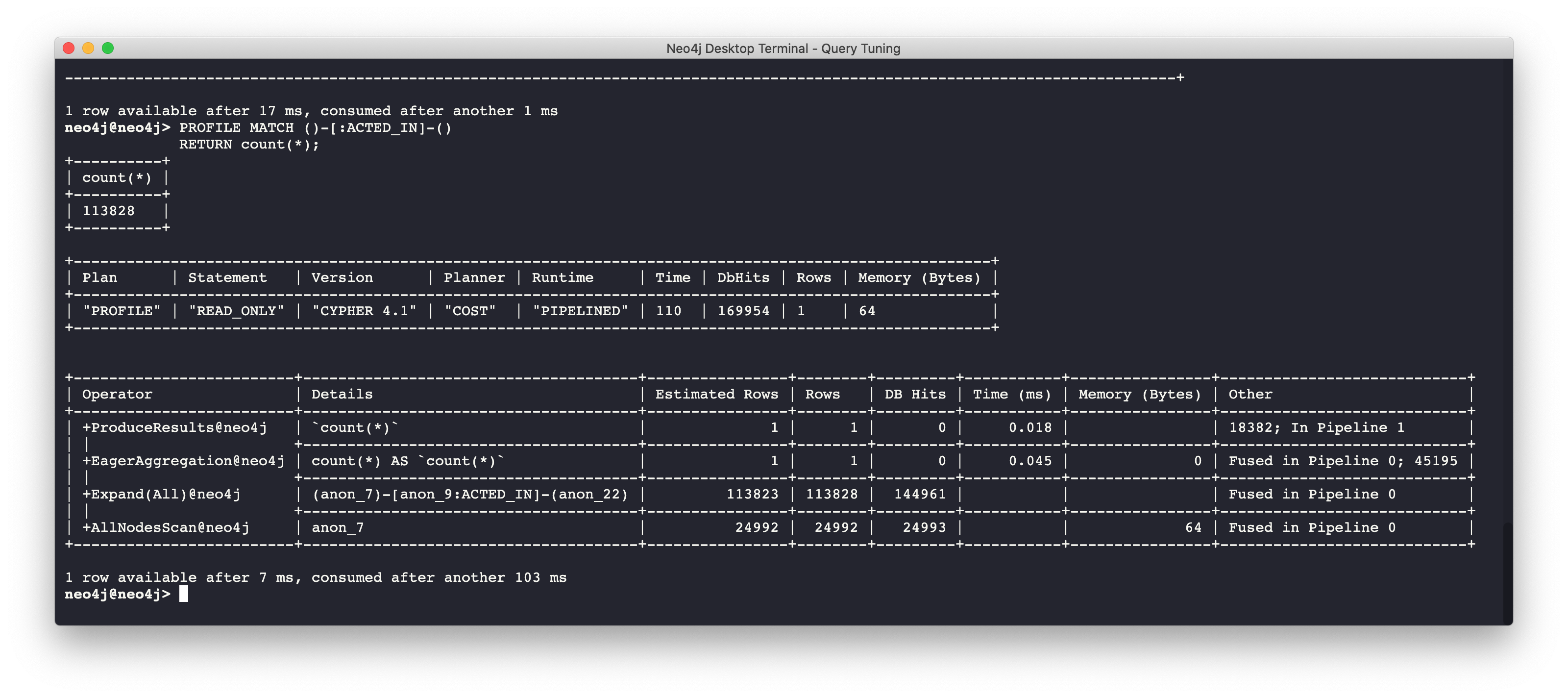

We see a retrieval of all nodes (24,992 rows), as well as a total of 169954 db hits.

Example: Count store is used

Here is a query where the count store is used, rather than retrieving the nodes and incurring db hits:

PROFILE MATCH ()-[:ACTED_IN]->()
RETURN count(*)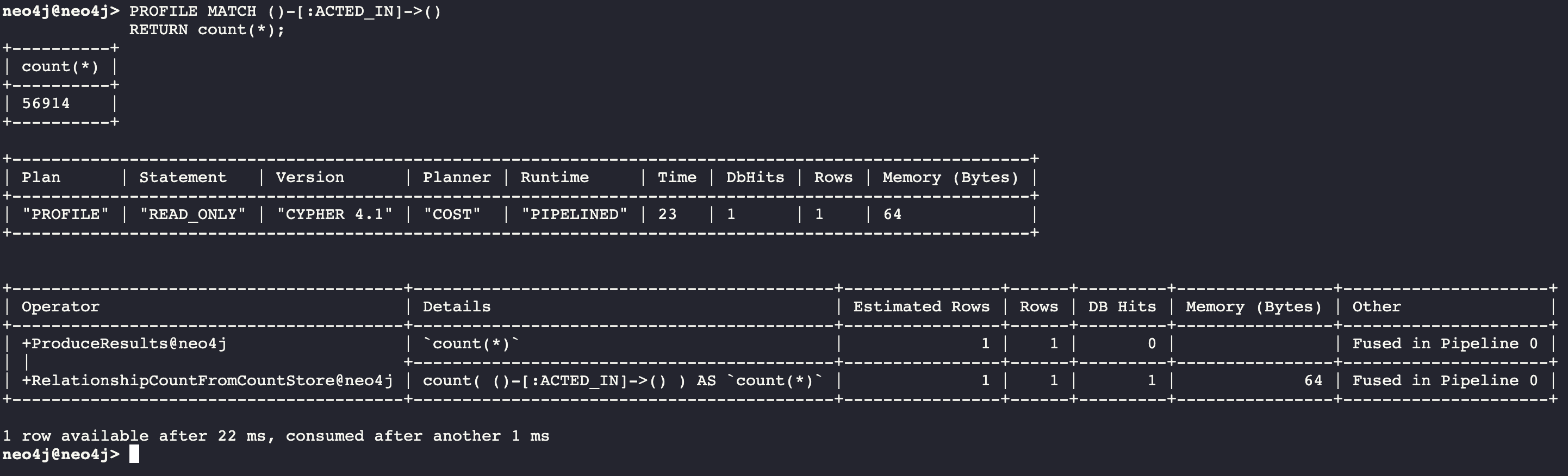

Seeing the RelationshipCountFromCountStore is a good thing for your execution plans.

Example: Is count store useful?

The count store is very useful, but not in all cases. Here is a query where we hoped to get some leverage from using the count store, but because we also need to retrieve the name of the person, there is a high db hit overhead:

PROFILE MATCH (a:Actor)-[:ACTED_IN]->()
RETURN a.name, count(*) AS count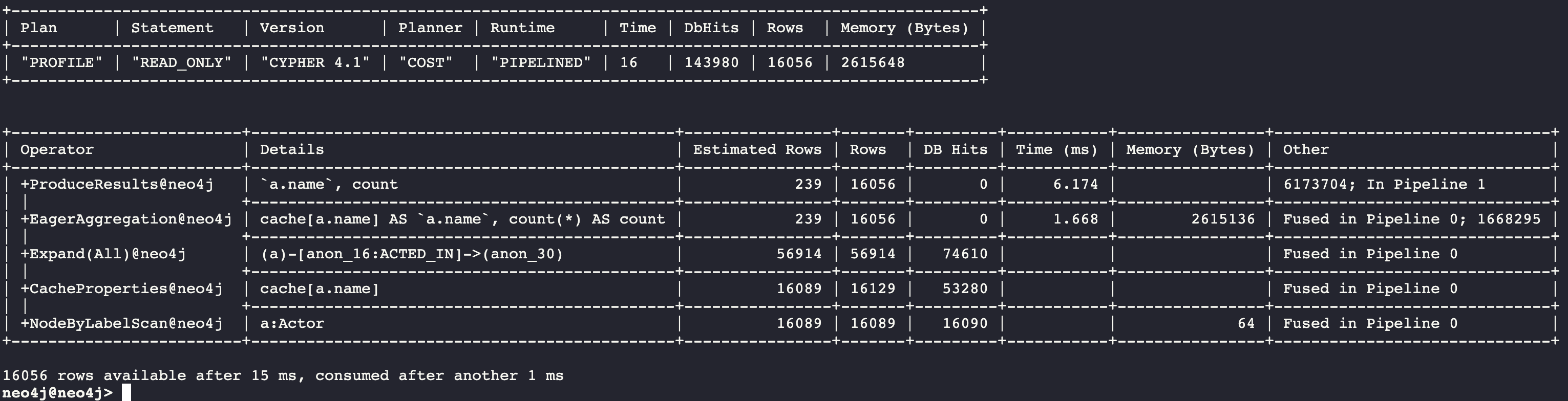

Here we see 143,980 db hits.

Example: Alternative to using count store

Here is an example we execute the same type of query,but the count store is not be used. We use size() to retrieve the number of relationships from each Actor node:

PROFILE MATCH (a:Actor)
RETURN a.name, size((a)-[:ACTED_IN]->()) AS count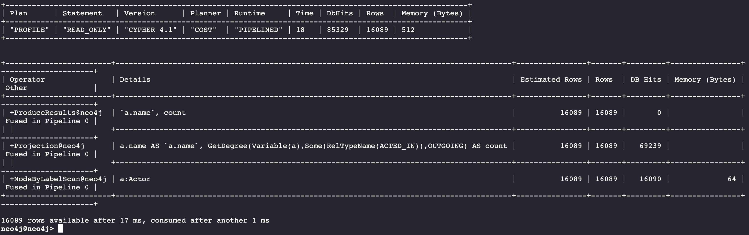

In this Cypher query, size() calls GetDegree(), which in this case, is more efficient than using the count store.

Controlling index selectivity information

Most DB Stats in the count store are updated with each transaction. The exception to this is information about the selectivity for each index value. Index selectivity is updated when a certain threshold of changes occur to the graph. You can control when index selectivity is updated, keeping in mind that more resources will be required if the index selectivity information is 100% synchronized with the indexes in the graph.

One way that you can control when this synchronization occurs is to adjust these settings in the Neo4j configuration:

dbms.index_sampling.background_enabled=true
dbms.index_sampling.update_percentage=n

Where the default used by Neo4j for the percentage is 5. That is, if more than 5% of the indexes have changes, then the index selectivity information is updated in the count store.

Controlling DB Stats (with Cypher)

You can also force the update to the DB Stats with these calls:

//update DB Stats for a specific index
CALL db.resampleIndex(':Person(name)')

//update DB Stats for all indexes
CALL db.resampleOutdatedIndexes()

Exercise 1: Answer Some Query Tuning Questions

In the query edit pane of Neo4j Browser, execute the browser command:

:play 4.0-query-tuning-exercises

and follow the instructions for Exercise 1.

This exercise has 9 steps. Estimated time to complete: 20 minutes.

Summary

You can now:

Describe the components of query processing.
Describe an execution plan.
Describe the cost of accessing nodes, labels, properties, and relationships
Understand the graph you will be working with:
- Data Model
- Indexes and Constraints
- DB Stats

Check Answers

Need help? Ask in the Neo4j Community