Analytical Subgraph Overlays in Neo4j

A common situation in Neo4j is to have a collection of dependency networks. Let’s say we’re dealing with company ownership structure, or which companies trade with other companies.

Usually companies have a large volume of this data across their entire customer base. But when you want to look at a single trading partner, the entire network isn’t relevant. You need to “zoom in” on one subgraph and see just the local parts affected by that trading partner.

To make this visual, let’s start with a picture of a small example graph and our ownership structure looks like this:

• A Company
• A Subsidiary
• Tiny Corp
• B Company
• B Subsidiary

And they’re all trading with one another, as indicated by the graph:



(If you would like to follow along in Neo4j Browser, the code that created this graph is here):

CREATE (a:Company { name: 'A' })
CREATE (b:Company { name: 'B' })
CREATE (aSubsidiary:Company { name: 'A Subsidiary' })
CREATE (bSubsidiary:Company { name: 'B Subsidiary' })
CREATE (tiny:Company { name: 'Tiny Corp' })
CREATE (a)-[:OWNS]->(aSubsidiary)
CREATE (b)-[:OWNS]->(bSubsidiary)
CREATE (aSubsidiary)-[:OWNS]->(tiny)
CREATE (a)-[:TRADES_WITH { value: 1000 }]->(bSubsidiary)
CREATE (tiny)-[:TRADES_WITH { value: 10 }]->(b)
CREATE (tiny)-[:TRADES_WITH { value: 11 }]->(bSubsidiary)
CREATE (b)-[:TRADES_WITH { value: 5000 }]->(a)
CREATE (b)-[:TRADES_WITH { value: 7000 }]->(bSubsidiary);

In a database of millions of nodes and possibly tens of millions of relationships, this tiny picture is one small island.

Let’s imagine that this is our island of interest, because what we’re trying to do is analyze the “A” Company and its dependencies.

Starting Point

What we want is an analytical sub-graph centered on “A”.

We know that we could build a simple version of this graph with a single Cypher query; for example, finding all of the relevant paths through the network, up to a length of three.

MATCH path=(startingPoint:Company { name: "A" })-[:OWNS|TRADES_WITH*..3]-(other:Company)
RETURN path;

For a first basic approach, we could change the nodes, labels and properties themselves to identify what we want to know. Let’s compute:

• Total net trading volume from a given company
• Distance from A to the company in question

If we knew those things, we’d know how important each company is to the total picture of Company A.

We can do so like this:

 
/* Calculate the distance from A to trading members, and tag them all with a "scenario" */
WITH 'My Analysis of A Corp' as SCENARIO
MATCH p=shortestPath((startingPoint:Company { name: "A" })-[:OWNS|TRADES_WITH*..3]-(other:Company))
WHERE id(other) <> id(startingPoint)
SET
  startingPoint.distanceFromA = 0,
  startingPoint.scenario = SCENARIO,
  other.distanceFromA = length(p),
  other.scenario = SCENARIO;
 
/* Calculate the total trade volume for everyone in the scenario */
WITH 'My Analysis of A Corp' as SCENARIO
MATCH (c:Company { scenario: SCENARIO })
OPTIONAL MATCH (c)-[r:TRADES_WITH]-(other:Company)
WITH c, sum(r.value) as totalTradeVolume
SET c.totalTradeVolume = totalTradeVolume;
 

Once we compute these simple attributes, we can now get a clean tabular view of our scenario, complete with many “graphy aspects” of it, as a table, like this:

MATCH (c:Company { scenario: "My Analysis of A Corp" })
RETURN c.name as name, c.totalTradeVolume as tradeVolume, c.distanceFromA as distanceFromA
ORDER BY tradeVolume DESC;

An Analytical Overlay

This previous approach works just fine. And since we’ve put these attributes as regular properties into the graph, we can use other tools like the BI Connector to visualize them and work with them via other technologies.

But there are some problems with the simple approach:

• We can’t really run multiple scenarios at once without them “clashing” on their properties.
• We don’t want multiple different analyses overwriting each other.
• We don’t want to modify the basic graph, because we’re exposing that information to other users. We may have security requirements where users are permitted to see certain company data, but not everything about our analyses.

The solution is to separate out this idea of a “Subgraph” and make it a new node unto itself. We can then connect that Overlay node to the rest of the graph, so we always know what our analytical scenario contains.

We do so like this:



The Cypher that computes this is a bit more complex, because we’re going to do both pieces (calculating trade values and distances) in one shot, along with creating the Overlay node, all in one go.

WITH 'My Analysis of A Corp' as SCENARIO
MATCH (startingPoint:Company { name: "A" })
OPTIONAL MATCH (startingPoint)-[spTrades:TRADES_WITH]-(:Company)
WITH startingPoint, sum(spTrades.value) as spTradeValue, SCENARIO
CREATE (overlay:Overlay {
  scenario: SCENARIO,
  created: datetime(),
  analyst: "John"
})
WITH overlay, startingPoint, spTradeValue
MATCH p=shortestPath((startingPoint)-[:OWNS|TRADES_WITH*..3]-(other:Company))
WHERE id(other) <> id(startingPoint)
OPTIONAL MATCH (other)-[otherTrades:TRADES_WITH]-(:Company)
WITH overlay, startingPoint, other, p, spTradeValue, sum(otherTrades.value) as otherTradeValue
MERGE (overlay)-[:CONTAINS {
  focusOfAnalysis: true,
  distance: 0,
  tradeValue: spTradeValue
}]-> (startingPoint)
MERGE (overlay)-[:CONTAINS {
  focusOfAnalysis: false,
  distance: length(p),
  tradeValue: otherTradeValue
}]-> (other);

Advantages of the Overlay Approach

• You never need to modify the underlying graph.
  This means that you can freely import/export data and change the underlying company graph, without interfering with analyses.
• You can express metadata about the analysis.
  Note that the Overlay node contains the created date, and the analyst who is interested in the work. Each overlay can get its own unique Subgraph ID, and then we can start asking more complex questions, such as “Show me the analyses done by John that are less than a week old, and that involve TinyCorp.”
• You can easily pull together the entire subgraph by traversing only one relationship.
  This is the Overlay CONTAINS relationship. Since we pre-computed graph distances, we don’t need to do those Cypher traversals over and over again.

Taking It to the BI Connector

Now that we have a simple schema focused on the Overlay node, we can now define a simple join in Tableau and pull data about all of the different overlays we’ve made, like so:



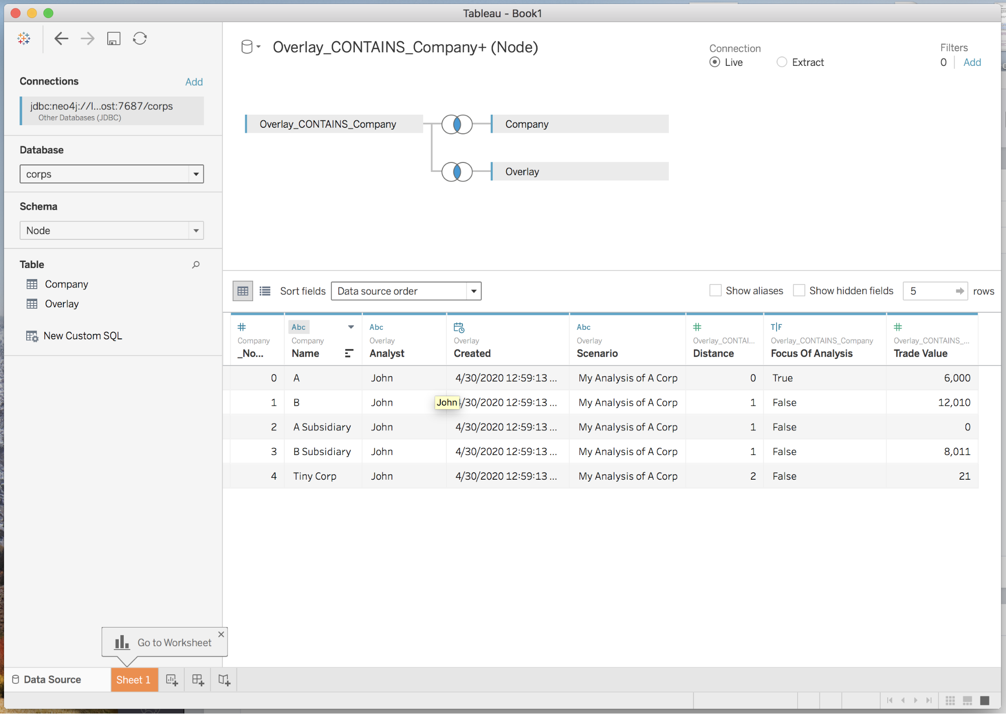
This is really looking at the same data as we saw in a simple tabular view in the “Starting Point” section. The difference is that we can now dynamically add different analyses to our graph in real time, and Tableau will always catch the updates.

And of course once we’ve gotten that far, we can build standard BI visualization on top of our data.

For example, we might build a chart that combines the distance from A with the total trading value of the relationship. In this view, we can see that B and “B Subsidiary” have rather large total trading values, and are “immediate neighbors” of A.





You can find more information on the Neo4j BI Connector here.

Conclusion

Many graph use cases call for doing specialized analyses on subgraphs of interest. Whether it is:

Dependencies between companies in a trading network

Software, networks, and servers in an IT infrastructure

Inter-related accounts in a financial fraud network or

Key customers in a retail scenario

The technique outlined in this article can help you pull the needles out of the haystack, and do custom analyses on one tiny island of data.

This is just another example of the benefits you get from “schema-flexible” graph data modeling, and Neo4j’s relationship-oriented approach. We hope this has been of help in adapting these techniques to your problems!