10 things you can do with Cypher that are hard with SQL

Head of Product Innovation & Developer Strategy, Neo4j
17 min read

Editor’s note: This presentation was given by Michael Hunger in December 2021 at Neo4j Connections: Graphs for Cloud Developers.
SQL has been around for a long time; it’s a powerful query language, but there are some things that just make more sense in Cypher. I’ll occasionally show SQL as a point of comparison, but in general, I will focus on the Cypher aspects because that is what we run here at Neo4j.
Before I jump into my list of ten things that you can do better in Cypher, I will first provide a little comparison of Cypher versus SQL, datasets, and graph patterns versus JOINs.
Cypher vs. SQL
SQL as a query language has been around more than 50 years and was developed with the involvement of many vendors and ISO committees. Initially, SQL started out as a query language for single tables. Later, JOINs and support for geospatial data for XML and JSON were added. Here is a typical SQL query which selects top-selling products from a retail database.
SELECT p.product_name, count(*) as cnt
FROM customers c
JOIN orders o ON (c.customer_id = o.customer_id)
JOIN order_details od on (od.order_id = o.order_id)
JOIN products p ON (od.product_id = p.product_id)
WHERE p.product_name LIKE '%G%'
GROUP BY p.product_name
ORDER BY cnt DESC LIMIT 5;
I used four JOINs in the SQL query to produce the following results.
product_name | cnt
———————————+—–
Guaraná Fantástica | 51
Gorgonzola Telino | 51
Gnocchi di nonna Alice | 50
Mozzarella di Giovanni | 38
Gumbär Gummibärchen | 32
As you know, relational databases are built on tables and connections are made by JOINs.
Cypher, on the other hand, is a language designed for graphs. For comparison, here is a query in Cypher.
MATCH (a:Person)-[:ACTED_IN]->(m:Movie)

WITH a, count(m) as movies WHERE movies > 2

MATCH (a)-[:DIRECTED]->(m)

RETURN a.name, collect(m.title) as movies, count(*) as count
ORDER BY count DESC LIMIT 5;
This query has the building blocks of a graph, meaning entities like nodes and their relationships are built into the code. Cypher is easy to read and understand, even for people who are not developers. It is a powerful, modern language and borrows from other query and programming languages like Python. Subject matter experts or business analysts can read these queries, provide feedback, or even write the queries themselves.
A popular feature in graph databases is that database searches are schema free or schema optional. That means you don’t have a fixed schema that represents your data, and you can instead evolve your schema data, adding new attribute types and relationships as you go. This makes it very flexible for developing an application.
Datasets
In today’s blog, I’ll be using two built-in example datasets in Neo4j: one called Movies and another called Northwind. We use an IMDb style database and the Northwind Retail database as examples, because there are lots of materials for those in SQL available. Here you can see the data models for both.

This is the movie database, and people have relationships to movies. They could have directed, written, produced, acted in, or reviewed a movie. The other database we will use, Northwind, has products, categories, and customer orders.

Graph patterns vs. JOINS
In Cypher, we look at visual patterns. Whatever you would draw on a whiteboard or on a diagram as circles and arrows, we are able to represent in the query language.
Nodes
All nodes or entities are in parentheses. You can also put stuff into the parentheses, for instance, a type of node or additional attribute:
()
(:Person)
(p:Person {name:'Emil'})
Relationships
Similarly, the simplest way to represent a relationship is just two dashes, but you can also add two dashes and a greater than sign for an arrow, or even use square brackets to add more information into a relationship:
--
-->
-[:RATED]->
-[:RATED {stars:5}]->
Combining nodes and relationships gives us Cypher patterns.
(:Person {name:'Emil'})-[:RATED {stars:5}]->(:Movie {title:'The Matrix'})
I can imagine seeing this drawn out on a whiteboard: a person named Emil, with an arrow pointing to a movie, titled The Matrix. All of these little half dashes are actually like a JOIN in a relational database. However, in a relational database we need to JOIN from your entity to the JOIN table and again from a JOIN table to the other entity, which adds computational steps.
FROM customers c1
JOIN orders o1 ON (c1.customer_id = o1.customer_id)
JOIN order_details od1 ON (od1.order_id = o1.order_id)
JOIN products p1 ON (od1.product_id = p1.product_id)
JOIN orders o2 ON (o2.customer_id = o1.customer_id)
JOIN order_details od2 ON (od2.order_id = o2.order_id)
JOIN products p2 ON (od2.product_id = p2.product_id)
WHERE c1.customer_name = 'Emil'
  AND p1.product_name = 'Philz Coffee'
This customer-product relationship SQL example here could be used to build a recommendation engine. To make a relational database work for this, you need many JOINs, each one slowing the application down. (As you’ve probably gathered, Emil really likes Philz Coffee.)
Now that we’ve covered some key points, we can dive into ten things you can do easily in Cypher that are difficult with SQL!
1. Path patterns
Path Patterns is an advanced feature to start with, but I thought we’d just go for it.
:param product=>"Pavlova";
Here I set a parameter called product to use a bit later in my queries. Now let’s take a look at the path patterns.
MATCH path = (p:Product {productName:$product})-[:PART_OF*]->(root:Category)
RETURN path
We have a product pointing to a list of categories. If you don’t know how deep your hierarchy of categories is, then you can just put a star and it will find arbitrary, linked relationships up to the root category.
MATCH path = (p:Product {productName:$product})-[:PART_OF*1..10]->(root:Category)
RETURN path
You can also limit this by saying find a path of up to 10 relationships.
Below is just one category, Confections, but I can add more categories.
MATCH path = (c:Category {categoryName: "Confections"})
CREATE (c)-[:PART_OF]->(:Category {categoryName: "Sweets"})-[:PART_OF]->(:Category {categoryName: "Unhealthy Food"})
RETURN path
Using a relationship type PART_OF, we add another category with a categoryName of “Sweets”. We can even add an additional category with a categoryName of “Unhealthy Food”. Here’s what our path would look like.

You can see this result goes all the way from my product to the root category. If I want to do the same in SQL, I need to spell out the query with all the levels and JOINs as far as I need to go. Alternatively, I could use a common table expression, but this is just a more complex way of joining tables together recursively.
Finding Loops
Under the topic of path patterns, another thing that you can do in a graph is find loops– for instance, if I want to see a loop that leads back to the same person again.
MATCH path = (p:Person)-[*1..5]-(p)
RETURN [n in nodes(path) | coalesce(n.name, n.title)] as path, length(path)
LIMIT 10
Here I am looking for a path of one to five hops, and I want to end up with the person I started with. This data can be shown tabularly, but also visually, which is what graph is all about. Here’s a longer loop with its visual.
MATCH path = (p:Person)-[*3..10]-(p)
RETURN path
LIMIT 1

2. Shortest path
The second Cypher feature is shortest paths. You’ve probably seen on LinkedIn that a person is so many hops away from this other person. This is something that can be done easily in a graph database.
:param name=>"Meg Ryan";
I begin with our starting person, and in our case I’ll use the name “Meg Ryan”. I want to find the shortest path from Meg Ryan to Kevin Bacon.
MATCH path = shortestPath(
    (:Person {name:$name})-[:ACTED_IN*..10]-(:Person {name:'Kevin Bacon'}) )
RETURN path, length(path);
I set the ACTED_IN linkages to be up to 10 hops away, and then I return the path and the length of the path. I can make this path an arbitrary length– one hop, two, three, four, five.

Here in the visual results we have a four hop path from Meg Ryan to Kevin Bacon. With our actor to actor relationships here, we have the movies in between.
3. Aggregation without GROUP BY
This next feature is something that I’m personally very happy about. I always hated GROUP BY in SQL because it is superfluous having to spell out grouping keys, both on the field selection and again in the GROUP BY statement. This is something that we wanted to avoid in Cypher because it is obvious if I have a GROUP BY statement or the non-aggregated fields grouping key.
MATCH (m:Movie)<-[:ACTED_IN]-(a:Person)

// in-between aggregation, only passing on declared fields
WITH a, count(m) as movies
// with filter on the aggregated value
WHERE movies > 2

// next query part
MATCH (a)-[:DIRECTED]->(m)

// aggregation at the end by a.name
RETURN a.name, collect(m.title) as movies, count(*) as count
ORDER BY count DESC LIMIT 5;
In this case, we find people that acted in a movie and then use an in-between aggregation. Using the WITH clause, we see the aggregation by person. Person is automatically our grouping key because it’s the only field that’s not aggregated in our return results.
4. Built-in data structure support: Lists and maps
If you come from a programming language background, it’s quite useful and common to use lists and maps as first class functions. Cypher has full support for lists. You can have ranges, maps, and slices. We have index access for lists, list comprehensions, and the quantifiers on lists. Along with conditions on lists, for maps we have dot-access, key access, and map projections.
// list comprehension
WITH [id IN range(1,100)
        WHERE id%13 = 0 |
        // literal map construction
        {id:id, name:'Joe '+id, age:id%100}] as people

// list quantor predicate on list elements
WHERE ALL(p in people WHERE p.age % 13 = 0)
RETURN people
This example of list and map usage is a bit contrived. We started with a range of 100 numbers, so from one to 100, we iterate over the list. Their IDs are in this list.
Then, because 13 is my lucky number, we add the filter and pick every 13 numbers, everything that’s divisible by 13 with no remainder. For each of those IDs, we create a map with an ID field, a name field that is a connected string with the ID, and an age field, which is the ID modulo 100. So we loop through people from one to 99. Here’s what this looks like.

5. UNWIND and collect
This next feature is something that I was involved in building, which is UNWIND and Collect. The Collect function turns a number of values into a real list. UNWIND is the inverse of that. Collect takes a number of rows and turns it into a list, and UNWIND takes a list and turns it into a number of rows. UNWIND is especially helpful with data creation and updates based on lists. If you pass in a list of data, such as a list of maps or arrays, you can iterate over this list of elements with UNWIND and for every element you can create or update an entity.
// turn list into 10k rows
UNWIND range(1,10000) as id

CREATE (p:Person {id:id, name:"Joe "+id, age:id%100})

// aggregate people into age groups, collect per age-group
RETURN p.age, count(*) as ageCount, collect(p.name)[0..5] as ageGroup
This example takes a list of 10,000 people, turns them into rows where the ID field is numbered 1 all the way through 10,000. Then, for each of those, we create a person with an ID.
For the inverse Collect function, we RETURN the age as the grouping key and then the count of how many people are in each age group. We can Collect any expression, including the person’s name, which we do in this case. Then we do a list slice on Collect to only show the first five values.

After running it, we see our age groups, one all the way through 100. Each age group has 100 people in it because 100 multiplied by 100 is 10,000. The lists are the first five people in each age group from the collection.
6. Pattern comprehensions & map projections
Neo4j has been looking at GraphQL, which is an API query language for graph shape domain data. About six years ago, we thought of some critical features in GraphQL that we could add to Cypher. One is called Map Projections, and the other is called Pattern Comprehension.
MATCH (m:Movie)

// map projection, with property access
RETURN m { .*,
    // pattern comprehension
    actors:
        [(m)<-[r:ACTED_IN]-(a) |
            // property access, nested expressions
            a { .name, roles: r.roles,
                movies: size([()<-[:ACTED_IN]-(a)|a]) }
        ][0..5], // list slice
    // pattern comprehension with filter & expression
    directors: [(m)<-[:DIRECTED]-(d) WHERE d.born < 1975 | d.name]
    } as movieDocument
LIMIT 10
For Map Projections, we use our Movies database, and then for a movie that we have to find, we RETURN all of its properties. That’s the .*, in the example above. You can then add other fields to this map as well. For instance, you can have an actual field in a map, which is a nested structure. This is good for when you want to RETURN a document-like element, such as with a front-end application or JavaScript application, and get a JSON object back with all the data in a nested document. Finally, Pattern Comprehension in the WHERE clause is similar to list comprehension, but for related graph patterns instead of lists of elements.
7. Combining reads and writes
If you’ve used SQL, you might have seen that you need to support Reads and Writes. You can do insert statements or insert from select, but that’s about it. This is why it’s nice to combine Reads and Writes in the same query. With GraphQL, while updating the database, you can also fetch data. In our example, just set the parameter with a movie title, a person’s name, and some rating stars. To query this parameter, we first find a movie through Read and then have a Write statement.
param rating=>({title:'The Matrix',name:'Emil Eifrem', stars:5})

MATCH (m:Movie {title:$rating.title})
// possibly write
MERGE (u:User {name:$rating.name})

// possibly write
MERGE (u)-[r:RATED]->(m)
// write
SET r.stars = $rating.stars
WITH *
MATCH (m)<-[:ACTED_IN]-(a:Person)
// read & return
RETURN u, m, r, collect(a)
If the User doesn’t exist, we create a User with the name ‘Emil Eifrem’. If the RATED relationship between User and Movie does not exist, we create it, and if it already exists, we access it. Then we set the new star rating. Here it is 5. After the update, we do another Read and find all the actors for this movie and RETURN our user, movie, rating, as well as all the actors from this movie. When I run this, here is the result below.

8. Transactional batching
If you do large updates on a database, you need to deal with the fact that in a transaction, the information in your update is kept in memory until you commit your transaction. Transactional Batching allows you to limit the amount of memory you use at one time.
:auto MATCH (o:Order) // imagine 100M
CALL { WITH o
    MATCH (o)-[r:ORDERS]->()
    WITH o, sum(r.count) as products, sum(toFloat(r.unitPrice)*r.quantity) as total
    SET o.count = products, o.total = total
} IN TRANSACTIONS OF 100000 ROWS
I want to compute two new fields from our total orders. For each ORDER, I get the number of products and the total price. The unit price multiplied by the quantity is our total price. We set these two attributes on the ORDER node. Here, you would make 100,000 updates for each sub-transaction. If you run this, you would see how the data gets updated in one transaction after another.
9. Built-in data loading: CSVs
In Neo4j, you can access CSV files via a URL and then use the CSV files to make updates to your graph.
WITH "https://data.neo4j.com/importing/ratings.csv" AS url

LOAD CSV WITH HEADERS FROM url AS row

MATCH (m:Movie {movieId:row.movieId})
MERGE (u:User {userId:row.userId})
ON CREATE SET u.name = row.name

MERGE (u)-[r:RATED]->(m)
SET r.rating = toFloat(row.rating)
SET r.timestamp = toInteger(row.timestamp)
I take a CSV file, and using my URL, I turn my CSV into a map structure. Each row is actually a map structure that I can use within my query tool. When a user doesn’t exist, we MERGE the user to create them. Here are the nodes this query creates for our movies, users, and relationships.

10. Built-in data loading: APIs
Here we have a user-defined procedure that can load JSON data straight from an API.
WITH "https://api.stackexchange.com/2.2/questions?pagesize=2&order=desc&sort=creation&tagged=neo4j&site=stackoverflow&filter=!5-i6Zw8Y)4W7vpy91PMYsKM-k9yzEsSC1_Uxlf" AS url

// load the json data from the URL
CALL apoc.load.json(url) YIELD value

// turn element list into rows
UNWIND value.items AS item
// deconstruct row data
RETURN item.title, item.owner, item.creation_date, keys(item)
LIMIT 5;
Using YIELD, we take the data and UNWIND it, turning this JSON list into rows.

We could actually also reach into this nested object and pull data out and even create a user from the nested fields.
Conclusion
That concludes my list of features in Cypher showing the many advantages of using a graph database over a relational database. I hope you give it a shot and try these features that aren’t found in traditional SQL!
Be sure to also check out these other resources:
The Cypher Refcard is a very handy reference for all the features of Cypher and links directly to the detailed Cypher Manual. We also have a GraphAcademy Training on Cypher with interactive beginning and advanced course offerings, as well as Cypher Developer Guides.
Share Article


Explore
Related Articles
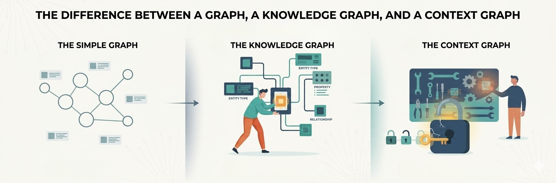
1 of 3: The difference between a graph, a knowledge graph, and a context graph
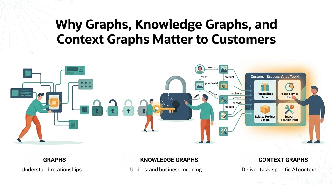
2 of 3: Why graphs, knowledge graphs, and context graphs matter to customers
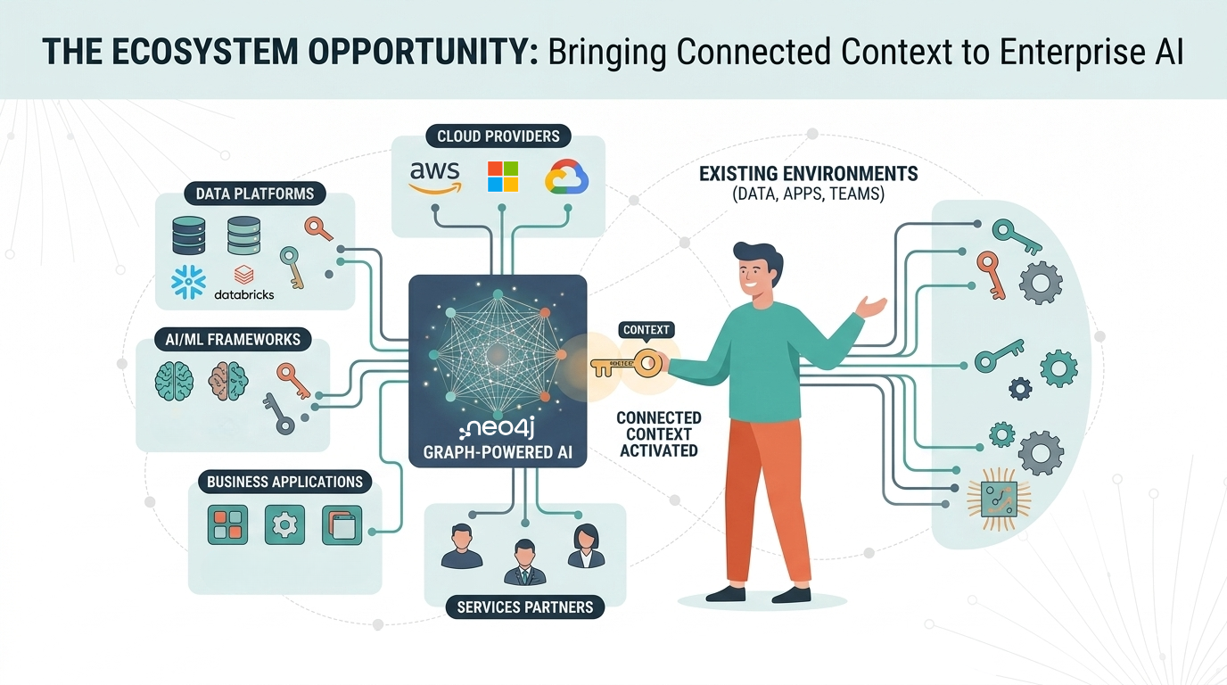
3 of 3: The graph ecosystem: Bringing connected context to enterprise AI