Presentation Summary
With challenging requirements in availability, scalability and global reach, Gary Stewart and Will Bleker at ING needed to reconsider their architecture by designing one that would remove throughput as a challenge, eliminate migrations and ensure consistency over time by means of redeployments.
In this post, Stewart and Bleker discuss the concepts they used when designing their architecture, such as pets vs. cattle (or trains vs. cars, as they call it at ING). They also detail their journey to NoSQL, which ultimately resulted in what they called the cache cattle pipeline, a paradigm they adopted to bring graph databases to life in their organization.
Furthermore, they delve into a use case for managing their Cassandra platform, including its architecture overview. Lastly, they share with us a few features and graph learnings they obtained from NoSQL thinking.
Full Presentation: Being in Control and Staying Agile with Graph Requires Shifting Left at ING
Being in control and staying agile with graph requires shifting left. I’ll break that title down in a few minutes, but before that, I want to give a bit of inspiration.
Below is my LEGO set, shown on the left. It’s called the Architecture Set Kit and it only includes white and see-through blocks. Specifically, it’s designed to help you abstract buildings away. You get to build up a building, break it down, find another inspiration and build it back up. This LEGO kit gave us a lot of inspiration for the architecture we’re going to be talking about.

To bring a little bit of the Dutch inspiration, there’s this beautiful building in Amsterdam, shown on the top right. It’s called the Amsterdam Eye, and it’s actually a film museum. I tried to make this building using the Architecture Kit. It took me about two days of breaking it up and building it. In the end, I was quite proud of my results (shown on the bottom right).
Going back to the title, being in control is all about security, data quality and availability/scalability. In the financial industry, we think we are unique in this, but in actuality, everyone needs to be in control of their data.
Staying agile, on the other hand, means obtaining new insights. Time to market is particularly important. For example, we get new features and need to build them quickly. This means our design also needs to take this into consideration.
We also need to have a pluggable architecture, and one way to manage this very well is to make a pipeline.
Being in control also requires shifting left, which isn’t a new concept per se. Shifting left effectively entails taking as much of your operational work and moving it to the design and build phases. This way, you do less on your operations side and start designing for no migrations.
One of the things we also realized is that systems are best designed not to last long. This will help you be more agile and more in control.
About Us
A short introduction: we’re Gary Stewart and Will Bleker. Gary is a data store platform architect and Will is primarily responsible for NoSQL databases within ING. Will is also the chapter lead for the events and data store team within ING, and takes care of platforms for Apache Kafka and Apache Cassandra data storage.
For those unfamiliar with ING, we’re a global financial institution based in the Netherlands, but we operate in over 40 countries worldwide with around 52,000 employees. Everything we do, design and build might be in Europe, but also has to work in Asia, America or any part of the world. Therefore, what we build needs to be easily adjustable and agile.
With that in mind, let’s get on with the post. We’re going to break it up into four main sections, starting with the concepts of how we think. Then, we’ll discuss the pipelines we use to actually make this work. Next, we’ll go into one of the use cases that we’ve used Neo4j in. As a final bit, we’ll show some of the graph learnings we’ve come up with in the last couple of months.
Concepts
Before I go any further, let’s briefly discuss the analogy of pets versus cattle.
Pets vs. Cattle
Back in 2011 or 2012, Bill Baker was struggling to explain the difference between scaling up and scaling out. He basically came up with the analogy of pets and cattle.
Pets are your unique servers. When you need more throughput from them, you generally scale up. These things tend to have a rather long lifespan.
But moving to the cloud, we generally move towards more cattle-like architecture, things that are disposable or one of a herd. Quite often, these are pipelined, so it’s simple to redeploy when something goes wrong. You scale them out and see that they’re mostly based on an active-active type of architecture.
The databases and the data stores that we support in our team – Apache Kafka and Apache Cassandra – fall mostly under this cattle type of architecture.
Our Twist: Trains vs. Cars
We kept screwing up and saying pets versus cats instead of cattle, so we decided to come up with trains versus cars as our own analogy.
When we look at our data stores, they’re just like the transport industry. In the last couple of years, they’ve gone through a couple of transformations.
There’s still a place for all of them, but in general, if we look at trains, they’re unique, long-lived items built on demand.You generally pack trains full of people, who all leave at the same time as part of a fixed schedule. If something should happen to this train halfway through our journey, then all the people on the train are delayed.
Cars, on the other hand, have gone from a manual to a fully automated process. They’ve become a mass-produced, consumable product. When something happens to your car – whether you’ve had a bad accident or it’s just old – you simply replace it for a new one, unlike a train, which has a bit longer lifespan.
In our IT landscape, we started noticing more and more that sometimes it’s okay for certain parts to not arrive at the same time. We needed that bit of flexibility and hence, we scaled out towards cars, because you have smaller amounts of people in a car. Should one car have a problem, only a part of your data will be delayed.
Our Journey to NoSQL
Our journey started from a relational database onto NoSQL, and this was quite a big mind change. We chose Cassandra purely for its high availability and scalability options. It also brought along things like tunable consistency, replicas and a whole bunch of other things that seemed quite daunting at first.
However, after using it for roughly four years now, we’ve grown so accustomed to how these databases work, as well as the added benefits you get from them. For example, lifecycle management has now become a breeze.
We’ve actually got a lot more weekends free, because in a typical master-slave, active-passive type of environment, you end up having to schedule downtime to switch between your databases. But, in an active-active solution like Cassandra, we simply do our patches during the day time now.
But, we now have some liquid expectations of any new technology that we want to adopt in the future in that the new technology has to follow these kinds of rules and features that we have. After all, we don’t want to go back to working weekends.
About a year ago, we noticed there was a big gap in our landscape that could easily be filled by a graph database in order to get to grips with our connected data. However, we didn’t want to go down the route of another active-passive or leader-follower type of solution, so we had to figure out ways to work around these challenges and keep our weekends free.
There were also other interesting observations: if you look at other databases, for example the key-value store, it’s quite easy to mess up a partition. In a relational database, you can mess up a table with a simple query. But, in a graph database it’s pretty easy to screw up your whole database. With these – and our weekends – in mind, we had to think about ways to work around this problem.
When you take any architecture, you always have a system of records. Generally, the path is that the demand or types of queries increase and then you start having performance problems.
What we decided was we were going to put a cache in between, as shown in the image below. That cache can be any database used to solve the problem, such as Neo4j, Cassandra or any other database.

Now, you’ve got a cache, but the data might not match if you get there, so then you have to build a batch loader or an export. This can be off-the-shelf tools (it doesn’t really matter), but however you do it, you have to manage that as well.
Then, of course, you need to build your APIs to use this cache database. Generally speaking, you don’t want to write in your cache – you normally just read from your cache and then write in your system records.
Finally, you realize, hang on, I only have data at a moment in time, so I need to add a real-time sync. So, we put the real-time sync in. This was a lot of work.
Then, of course, you start noticing that we also need a resilience pattern between each component, so that the APIs are resilient on the cache databases. Moreover, the cache database, batch loader and real-time sync have to be resilient. It gets more ugly when you want to be in multiple data centers.
In this way, you actually start realizing that lifecycle management is hard. Each thing has versioning and requires cross data center resilience. We decided we didn’t really like this very much anymore. Again, this is a per-use case, so you have to figure out what fits where. But, we decided that we needed to simplify this.
What if we were to put all of these components into one car and manage that on its own? This way, we wouldn’t have APIs calling different incidents of databases.

Here, you get comfortable with rebuilding – you actually have all your code there to rebuild fast. You also don’t have to do migrations, and if you want to do availability, you just deploy an incident in each data center. This is a lot easier to reason with. When you’re using technology like Neo4j, all the data must fit on one node anyway. In this way, you’re actually not more restricted than before.
This is all fine and well, but we can actually make this even more simple, as shown in the image below. When you use Kafka, which has features called compact topics, you can get rid of the batch files and then use compacting topics to design that away, because managing files is also a security place. Then, you have to build in all the mechanisms for that.

We’re not going to go into too many details about Kafka because that’s a separate post on its own, but just know that you can design the components and even take some components out by using Kafka.
You can even take it one step further, as shown below. We like cars, we see Kafka as a car and our cache database is also a car. A lot of use cases can actually use Kafka or any other technology for a system of records. Then, you can get comfortable with a materialized view.

When you break a database down into two parts – a commit log and a materialized view – you basically use one technology for the commit log and another for the view of that data. Now, we’ll talk about how to build that up.
Pipeline
We’re building a whole lot of things here. We want to build them a lot, and quite often. So, how do we do that? Well, first of all, let’s put a pipeline in, because we don’t want to be building things up manually everyday.
In the example below, we’ve got two cars running. The car is the consumer on the one side, with the batch loader, the real time sync, the API for the customers and also the Neo4j database. This can run in a docker container, a VM or whatever technology you use within your company. The load balancer on the right hand side basically distributes the load across these two machines.

Let’s say we’ve got a new feature, or one of the cars broke down and we want to put a new one in. We can add a new VM or docker container, block all the ports to make sure that no client connections can come in and query the database or application while it’s being built up.
The second step is to get all the artifacts, libraries, binaries and everything else you need to build up a car. Similarly, in the car industry, they make sure they’ve got all the components in the factory to build up a car from A to B.
Then, we start with a pre-processing phase, where we source all of our data from the system of records, which is Kafka on this side. From there, we convert the data into whichever format we need (in our case it was a CSV file). We then use the Neo4j admin import tool, which I’ll cover next, to import the data into our application, or our car.
We can then start up the database, and after that, we’ve got a couple of post-processing steps, which includes things like creating indexes and running other complex queries to start up our applications and the rest of our car.
Once that’s all done successfully, we unblock the ports and perform the switch. We take out the old one, and the new one’s running without any downtime for the application.
Neo4j Admin Import
So, I touched briefly on the admin import above, but now we’ll go more in-depth. Admin import is a key tool for when you want to rebuild quite often.
In this example here, we’ve got a simple model with a source, which in our case was a host. We also have a server, and we’ve got a bunch of messages that come in and relate to this source.

Here, you’d use the admin import tool, as shown below. Do note that this can only be used once when the database is still empty because it bypasses the transition manager, and that also gives it the speed in importing loads of data.
So, we import two CSV files with nodes, the sources and the messages, and then a third one with all the relationships.
Here, the nodes have an
ID, a name and a LABEL, as shown below. The relationships you need are a START_ID, an END_ID and the TYPE of the label that you’re importing. 
We ran this on our use case and managed to import around 11 million nodes and relationships in just over four minutes. This is quite good, especially if you’re rebuilding frequently. But, seeing as we started rebuilding four or five times per day, our clusters and environments kept on growing and getting more and more data. We needed to optimize this.
Basically, in a third of the time, we managed to import more than double the amount of nodes and relationships. This is shown below.

An easy way to get that was to change the names of the IDs, as shown on the right. An ID is only used during the importation – it’s not real data, so just make sure you don’t have duplicate names there. If you work around that problem, you can decrease the size of the file. Hence, the amount of data coming through the admin import tool dramatically increases in your performance.
Use Case: Managing Our Cassandra Platform
Our particular use case was for managing our Cassandra platform. It’s not the first place you would think to use graph technology, but we wanted to stay in control of our clustered environments.
We started playing with graph with Neo4j about a year ago, and we manage our Cassandra environment that consists of a multitude of nodes and clusters. On those clusters, we again have loads of customers that all consume key spaces. We know there are lots of numbers, clients, components and other departments within our company that we have to deal with, but only when you start putting data into a graph database are you able to visualize it. From there, you realize how many components you actually have to deal with.
Now, this is pretty much business as usual, because every company has rapid growth and dependencies. But, we wanted to stay in control of our clusters. What we were seeing was that as soon as an instance occurred on a multi-tenant environment, we had loads of customers on our environment, all with their own needs and use cases.
Moreover, if something happens on one of our clusters, we would see the operators log into a multitude of nodes, run all kinds of queries to find where the problem is, look at all the different components and try to – in their own heads – belay the links between the problems.
We thought there must be a better way for this and wanted to pipeline this. Because we didn’t value initial bursts of energy anymore, we needed to pipeline our heroes and find a way to work around this problem.
Architecture
What we did was create this simple architecture, where we have a producer on one side, a queue in the middle and a consumer on the other side.

The producer is something really simple and efficient. It’s a small binary that runs on all of our nodes, and basically runs all of the commands that the operators would do once they log into the machines to try and get information about them.
The producer produces just raw messages. They don’t do any filtering or fancy things on the producer. All the raw events are pushed onto the Kafka topic and consumed by the consumer on the other side, who’s a much more complex piece of technology that does all the parsing. There, we do all of the parsing of the rules and data.
In the image below, we’ve got our producers on the left side running on all the nodes. Should we need to add new commands, we just need to run a configuration file on the node that contains a list of commands and dictate the interval at which we want them to be run. These raw messages can then be put onto a Kafka topic.

On the other side, we’ve got the materialized view: the “car” part of our architecture that we explained earlier. The consumer reads it, transforms the data into the format we can use for Neo4j and imports it into Neo4j.
Before we have an incident, we still need to manage the configuration for certain aspects of our car. We store this in GitLab. The consumer then consumes from both Kafka topic and GitLab to obtain the state of what they want their environment to be.
Now, when they get an incident on their environment, instead of logging into all the nodes and trying to find relationships between different components within the environment, the operator can now log into the Neo4j database. They can do so either via the web interface, Python script or whatever method they choose, and run queries to find relationships between different components.
All of this grew quite fast and we empowered a lot of people with this, where everybody had their own Cypher queries. This became a bit unmanageable, because we still had heroes, the guys with the Cypher queries.
So, we ended up going for an option using GraphGists. We would copy and paste commands and it would run. But, it’s useless if five people keep running the same commands everyday. So, we thought, let’s stick that into the consumer, ask the consumer to run these commands every 10 minutes and output that to a static HTML page. In this way, when something happens in our environment, you don’t need heroes with Cypher queries anymore – you simply need someone who can look at an HTML page.
Now that we have all this data, set the rules and stored a bunch of configurations of values and thresholds for our environment in GitLab, we can also start putting alerts on them when processing them.
Through this process, we’ve gone from a simple producer to the consumer where everything is parsed and even produces notifications to the end points.
Consumer: Graph Model
If we narrow down into the consumer – because the consumer’s not only where a lot of the logic is, but also the one that gets rebuilt all the time – we would have to parse the message. Because we’re doing nothing on the producer side to parse the message, we leave that to the consumer. This is the first step.
Generally speaking, you’ll want to parse, though you might have to change the rules later if you have new insights or want to take some more data out. That would normally break down to key-value pairs, which we can get into the graph database very quickly. A message on its own is mostly meaningless, but one combined with all the other messages from other hosts, machines and message types holds value.
Once you have your data in the graph database, you can start doing observations, calculations and recommendations, because you can now automate this. We started doing this repeatedly, and while we were doing this, we came up with a few principles that helped guide us to build this correctly.
One main principle is that you definitely need an inventory. You need a system of truth and you need to know what you’re looking for. If you have a self-discovery system, then you can always find out what’s going on. You have to have expectations so you can check what’s going on.
Second, you need to define agreements in code. If you can’t make agreements in code and have that checked once it’s deployed or rolled out, then it starts becoming very difficult to check. Every agreement – such as configuration for types of clusters – needs to be put in code so that you can actually use them in your graph model.
We’ve been doing databases for years and one of the things we don’t like about graph, sorry Neo4j, is it’s schemaless at the very minimum. On one hand, we love it, and on the other, we hate it. Schemaless tends to not allow you to document the data model, and requires you to have another tool if you’re rapidly building stuff. So, we actually ended up documenting a data model.
This is something we had never done. One of the things that we found missing is that you can’t easily add comments or metadata about the model in the graph – or at least we haven’t found out how to do that yet.
So, another key principle is that you need to get into the comfort of rebuilding, since no data migrations are allowed. When you repeatedly rebuild your model, the next person who comes into the project will be able to learn that project very quickly, because they now understand how things get to where they are. Because a graph model is very functional, you not only need to understand graph as a technology, but also understand the data that you’re working with.
So What Happened?
What actually happened was we wanted to learn graph. We weren’t really fully convinced it was the best fit for our use case, but it actually turned out to work really well.
Where did this actually come from? We started with four or five commands in the producer, and within two or three months, we ended up adding 50. This happened so quickly because we were like little kids in a toy store getting data out, linking stuff and figuring out what we could add.
Then, we would keep adding configurations to the producer and the momentum was going so fast. We even, for example, put net stats information and tried to check which applications were connecting to the cluster and whether they were connecting to all the nodes correctly. By just looking at the behaviors of the operational data, we managed to find misconfigured customers.
From there, we realized our architecture helped us with this way of thinking. Because it became easy to rebuild, we created a learning environment for learning graph. It took us, since we started, over 300 cars that were destroyed and rebuilt to actually learn how to use graph and obtain all our findings after each iteration.
Graph Learnings from NoSQL Thinking
This moves us into the last section.
The first feature we’ll discuss is one of the lesser-known features. Traditionally, when you get a message, parse it and try to get that in the database, you would have to write
SET and “property name equals,” and you’d have all of these long lists. However, there’s actually something called “SET equals,” and after that, you can use a map. Then, if you use a +=, you can get all of the properties in one go. This way, you don’t actually have to mention the list that’s mentioned in the WITH. 
The reason why this is also interesting is because now we can change the parsing rules without having to change the data going into Neo4j. Essentially, you can break everything down to key-value and then get it into your database and write your queries. If you change the parsing rules, then the raw data also changes and you need to rebuild. That’s something we did quite often, so we simply rebuilt and destroyed the old instance.
Let’s move onto the next feature we learned. As we mentioned above, we actually started documenting a data model, which is shown in the image below. It’s blurred out, but I wanted to point out that the blue source is in a different place in my model than the yellow source. The two are not the same.

Because we were building so fast, we’d add another label or node and kept adding and adding. Then, we accidentally realized we used the same labels for two different objects. So, when we did
CALL db.schema(), we’d get a weird linking mess. That’s why we documented the data model to make sure that we don’t make these mistakes again. What are solutions to this? You can use the property existence feature, which protects you in a lot of cases. However, in the Cassandra world, we always say you need to solve your reads with your writes. Overall, you have this theme where you can simply fix code and rebuild or destroy the incidents.
Now, let’s look at a very simple model, a source
HAS_MSG. 
It’s not rocket science, but what we forgot here was that we were suddenly adding 50 produced messages every hour. Over time, the number of nodes attached to the source was very large. We’d always joke that if you’re too scared to open the node or expand it with the browser, when you press plus and your browser starts getting a little bit wobbly, then you might want to rethink traversing to reduce the density of the nodes.
So, how would you do that? Instead of having a source
HAS_MSG, you can then say that a source has LAST_MSG, has PREV_MSG, has PREV_MSG, has PREV_MSG and so on. 
In this use case, we mostly cared about the last message, not all the other ones. Though we needed them, they weren’t the main driver. We actually learned this at a presentation in GraphConnect London. We came back to our office, simply changed our code and rebuilt.
Finally, we talked about never doing a migration. At first, we thought we might as well attempt a migration because there was no point in saying migrations were bad if we’d never actually tried. And we’d often write the following query:
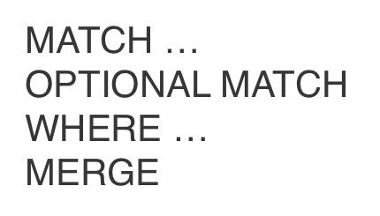
Every time I wrote one of these queries on the database, I’d basically have to rebuild and destroy the database. Essentially, the outcome of this is that I’ve destroyed my database, purely because of one simple mistake. The problem with
WHERE being after OPTIONAL MATCH was that you’d get a bigger dataset and effectively do a lot of stuff you didn’t intend to do with the first query. Instead, we needed to modify our code to look like this: 
Conclusion
We started off this post by saying that in order to stay in control and be agile with graph, you need to shift left. Shifting left is not an easy thing to do and requires a lot of upfront work, but once you nail the shift left and design for rebuild, you ensure agility.
By enabling the rebuild feature, you can simply add new features as often as you want and just rebuild. You create a learning environment in which people aren’t afraid to make changes because if their change didn’t work, they can simply rebuild to the old version.
Ultimately, this ensures that you can keep control over your environment. The more often you rebuild your data, the better your data quality will be. You don’t have to work with data migrations, so there are no places to mess up your data. Moreover, when you wanna scale out, you simply spin up X amount of extra nodes. That’s how we stay in control of our environment.
Think you have what it takes to be Neo4j certified?
Show off your graph database skills to the community and employers with the official Neo4j Certification. Click below to get started and you could be done in less than an hour.
Get Certified
Show off your graph database skills to the community and employers with the official Neo4j Certification. Click below to get started and you could be done in less than an hour.
Get Certified