The secret sauce of Neo4j: Modeling and querying graphs

Field Engineer
28 min read

Editor’s Note: This presentation was given by Max De Marzi at GraphConnect New York in September 2018.
Presentation summary
Welcome to the world of graphs. If this is one of your first visits and you feel like you don’t quite understand what graphs are all about, then continue reading this post.
First, we’ll get down to the basics of Neo4j, breaking down the property graph model and delving into how Neo4j differs from traditional SQL databases.
Then, we’ll introduce the one slide – the secret sauce of Neo4j – that you must understand. Along with that, we’ll explore modeling by looking at examples on modeling flight data, building a news feed and constructing a recommendation engine.
Full presentation: The secret sauce of Neo4j
My name is Max De Marzi and I’m a Neo4j Field Engineer. I blog about Neo4j and all kinds of crazy things you can do with it. I also go to different customer sites, where I help them solve their problems and build a graph solution.
This post is mostly about three corners of my experience with Neo4j, but what matters from this post is that you click out thinking about graphs. You have to drink the Kool-Aid, become a graph person, make it a part of your lifestyle and forget about all the other bad databases that exist out there. That’s my goal.
The property graph model
Let’s first talk about a property graph model, which is where things start. In graph databases, we don’t have tables, columns, rows or foreign keys. Instead, all we have are objects floating around in space, connected to each other by relationships that are directed and have types.
For example, we see here that Mary drives the car; the car doesn’t drive Mary. Also, Mary loves James and he loves her, but that doesn’t necessarily have to be the case.
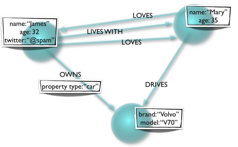
Moreover, the properties can be different. Here, we have two people or user nodes, but James has a Twitter property while Mary doesn’t. That’s also perfectly valid.
The other thing to notice is that the relationships also have properties, unlike the triplestore or RDF model, where relationships don’t have any properties. We also have labels; nodes can have one or more labels that identify what kind of node it is. These labels are optional, but nowadays everyone generally has at least one label on a node.
What you (probably) already know
If you come from a SQL background, you probably already know a lot about tables.
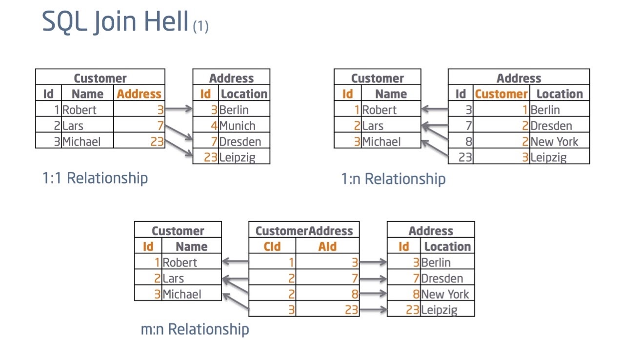
Say I have a customer with an address. With SQL, I’d have a customer table and an address table, and I’d connect the two together with the foreign key. Everyone’s happy.
But that’s not all that happens in the real world. For example, if a customer can change an address, I’d now need to have a pointer going the other way from the address table to the customer table. But, one address can have multiple customers and one customer can have multiple addresses, and it gets a little messy, so we utilize a join table. This gives us a customer address table that points both ways. It has no practical value except providing the foreign keys where it points to.
In this way, if I wanted a query on how this data is related, I’d have to perform some kind of join. And that’s the way we’ve been doing it for more than 30 years in SQL. The problem here is that every time you want to know how things are connected, I’d have to execute that join. What that really means is that I’d need to find those foreign keys, see where they’re connected and follow them through.
How do you find the key in a relational database? Well, I’d have to use an index. And if my database people did their job properly, everything should be nicely indexed, meaning that I’d have a B-Tree in the database. A B-Tree’s is a log n data structure, which means as my data grows by 10, speed only slows down by two. This means we can get pretty big before encountering problems.
But, the problem is that we already got to that large size. With this big data, we’re searching for more keys, meaning we get slower and slower performance. The more joins and look-ups for keys we have to do, the worse things get. We start screaming at our database to go faster – and that’s usually when we transition to NoSQL.
Same data, different layout
The folks at Neo4j took the same data you had and gave it a slightly different layout. Let’s look at some conference data:
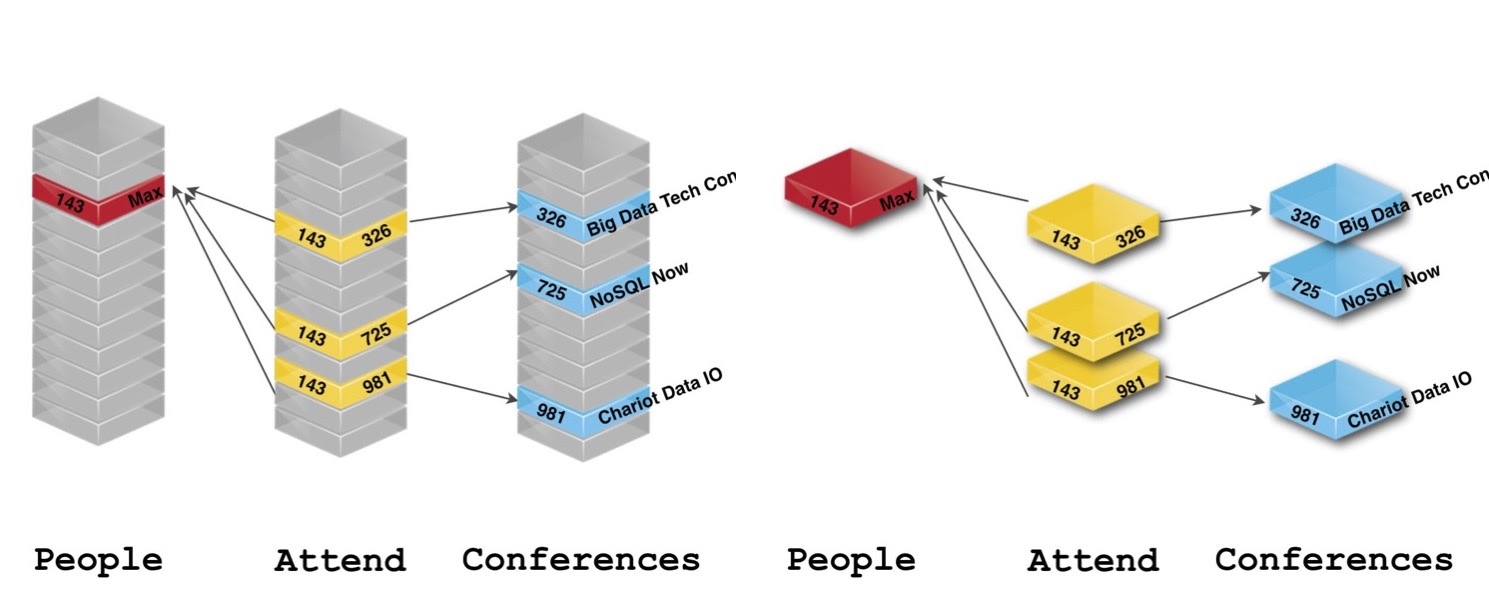
If we’re only focused on which conference Max, for example, attended, we realized we didn’t don’t care who the next person is or what other conferences exist in the tables. All I care about is the relationships between everything. Its data is still there, we just don’t need tables to handle this. Instead, we use nodes and relationships.
Relational databases
Even though they’re called relational databases, they really can’t handle relationships. As you add more and more relationships to your relational database, it gets more and more complex, and it starts looking crazy. Sometimes, you’ll walk into a DBA or developer room, see ginormous ERD diagrams that take up the whole wall and you’re supposed to understand what’s going on with that. It’s very hard to do. Again, as your data grows with the number of joins and you try to execute a table join that’s 15, 20 or 30 levels deep – forget it. It’s not going to be a good time.
SQL was built so many years ago around Set Theory, not graph theory. So if the data feels, smells and tastes like a graph, using SQL on it is the wrong thing to do. (Don’t get me wrong: SQL is great if you have nothing but tabular or set data.)
Moreover, SQL isn’t very flexible, which means that you have to know your schema before adding any data.
NoSQL databases
To fight these problems, a bunch of vendors got together under the moniker of NoSQL, which includes the following major categories:
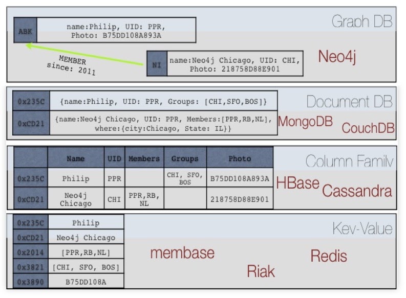
Starting from the bottom, we have key-value stores, which helped fix the join problem.
Next, we have the column family, which says: “Listen, we’re going to pre-join everything for you, duplicate the crap out of your data and you’re going to buy 100 servers from us. So we’ll make lots of money.” In many cases, you’ll end up with thousands of servers at Apple running Cassandra and stuff like that.
Document databases say: “That’s a horrible idea. We have a better idea. We’re going to take everything we know about an object and squish it all together.” This is fine, unless you want to know how these documents are talking or connected to each other.
Last, you have the graph database saying: “Let’s take relationships and make them first-class citizens. We’re going to store them on one disk and keep them up in memory. They’ll be physical, real things in our data.
Now, the bottom three categories – document stores, column stores and key-value stores – typically aren’t ACID; they’re non-transactional, though some have started to announce that they’re becoming proper ACID databases. Additionally, most of these can’t handle relationships very well.
What’s Our Secret Sauce?
Our secret sauce is here. If you have no idea what graphs are or what Neo4j is about, this is the thing to remember, though it’s not a perfect, physical description of how it works, but rather a slight extraction.

Basically, what you have is two giant arrays: one array of nodes and one array of relationships. Every record in the array is fixed in size, so you’re actually looking at one single node and one single relationship of the tree.
Furthermore, every node knows what types of relationships are connected to it. Let’s say we’re looking at a social network and you have to be in Node One. The node knows it has friends relationships that happen to be of Type One. If we want to get all their friends, we can go to the Type One relationship and ignore the Type Two and Type Three relationships.
Then, every relationship type has two lists – incoming and outgoing – that contain relationship IDs, which are basically relationship pointers. What’s nice about this is that every type list is stored by node, so whether you have a thousand or a billion people in your graph, getting through 150 friends costs exactly the same. You essentially jump to the node you care about, traverse the 150 relationships and you’re done. All it cares about is what you’re looking at.
However, we pay a price: the joins are done on creation. What happens every time we create a relationship? We need to go to the first node and add an item to its list in the outgoing direction. Then we go to the node that’s receiving the relationship – to the list of incoming – and we add an entry there. After, we go to the actual relationship object and save its direction, and also add some properties if necessary. In this way, it costs us three, rather than one, to add a relationship to Neo4j. In contrast, in a relational database, you go to the join table, get an entry with two numbers in it and you’re done.
But an upside is that we get the joins for free. Everything is done by an array, so there’s no hatching, look-ups or indexing. Everything is done directly by O1 access, by looking at the next array. These relationships just store an ID, which points to the record.
If you get this, you’ll understand what Neo4j is about, regardless of size. It’s just a matter of traversing relationships using arrays. There’s no magic to it – you can build this in a weekend.
Real-time query performance
What this provides are very fast queries for some use cases, but not for everything. Like many databases, Neo4j is good at some things and terrible at others.

Let’s go through some bad queries. Imagine you have the data of every actor in Hollywood with everyone’s height property. Say you wanted to figure out the average height of all of the actors. That’s a terrible query for Neo4j, because we’d have to jump around random nodes looking for those actors. The first node could be an actor, the second node could be a movie, the third movie could be a commercial, the fourth node could be a play – who knows? Obviously, you might have labels that tell you where the actors are, but you still need to jump around quite a bit.
Next, you have to find the height property. Some actors might have the height property as their first property and some might have their height property as their last, because nodes can have any number of properties, in any order whatsoever. All of this is going to cost us a lot more than a relational database, which can just go to the actor table and do a scan, or a column sort that can go into height, go across and figure out the average. This is a better query for Cassandra than anything else.
However, if you wanted to know how these actors were connected to each other by the movies that they were in, then that’s a perfect query for us. Same data, but a different use case and query. If you care about performance, you want to take all of this into account.
Reimagine your data as a graph
It all works as long as you can reimagine your data as a graph. You’ll get better performance if you’re not only looking at sets of data, but also its relationships.
Cypher was built for graphs, so it’s really easy to explain what you’re trying to do with a language like Cypher. However, if you can’t do it with Cypher, you can do it with Java, Gremlin or other languages that work with Neo4j.
Moreover, Neo4j is flexible and consistent – you can add data, nodes and properties on the fly. It’ll figure out whether something’s a string, a number or a user. Neo4j will just store it as whatever you give it; it’s schema-optional in a way. This works really well for proof of concepts or when you have a greenfield idea and not sure what you’re going to build.
But, it’s also consistent because we have real transactions. You can start a transaction, make a thousand changes to the graph all over the place and at the end decide to commit or rollback all of those changes. In this way, it’s very similar to your relational database.
Modeling
This is where things get weird. If you know the third normal form or traditional database modeling, you’ll need to unlearn a few things.
Of course, there’s the normal way of doing it, and we always tell people this first lie: that graphs are completely whiteboard friendly. And they are – if you want to go slow. But if you want to go fast, you need to get a little more creative.
Some models are easy, like this one:
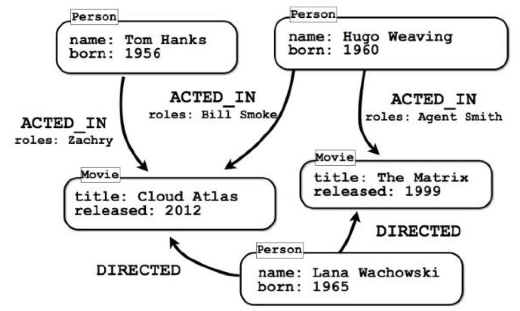
If you wanted to know who played James Bond, this is a terrible model for that query, because there’s no quick way to get to it. You’d have to rip out the actor or character, turn that into a separate node, find the James Bond character and figure out who played that character and what additional movies they were in. In this way, the models and the queries have to align. It’s not like the normal form where this is the right way to model things, and we’ll just figure out where the queries are later; you have to build it from both sides. You need to build it from the data you have, the queries you’re asking and match the two together to get the right answer.
Flight data
I’ll quickly go through another example of how to model flight data and airlines. You could model it like this:
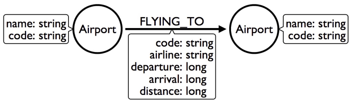
We have an airport – with a name and a code – as well as a flight to another airport, who has its own name and code, and we’ll stick everything about the flight into the relationship.
Let’s say I want to build a flight search engine, and want to find flights from New York to Chicago tomorrow. This is a horrible model for that because I’d have to look at the JFK airport, find all the flights for the whole year, look for the ones that are tomorrow and see which ones are specifically going to Chicago. That would take forever.
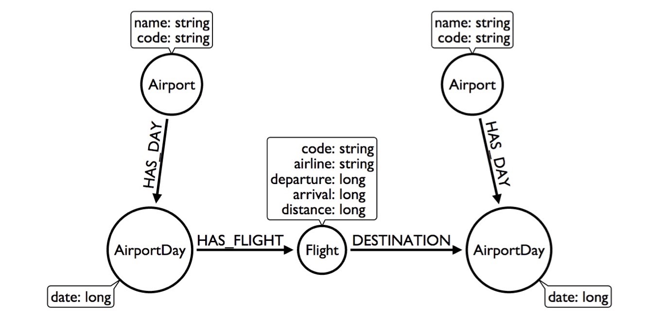
Another thing we can do is make flight a node. That way, the airport has a flight, the flight has a destination and we’ll stick with the properties in there:
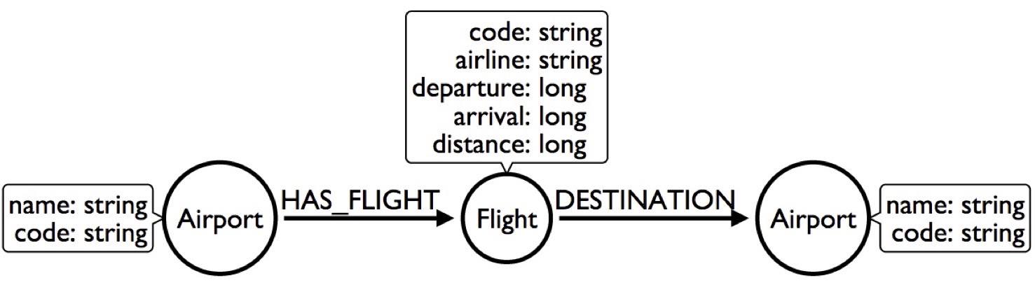
Okay. Things got better but didn’t get any faster. In fact, it’s actually slower, because now we have to jump through two nodes.
So, we have to get creative. Well, people are gonna be searching by date, so we can take the airport model and say the airport has days. Every day has flights, so instead of looking at 300,000 flights in a whole year, I can just look at the 1,000 flights in a single day:
This made my query better because now I have to look at less of the graph. But, we can still do better than this. Instead of having the HAS_DAY relationship, we can actually put the date as the relationship type.
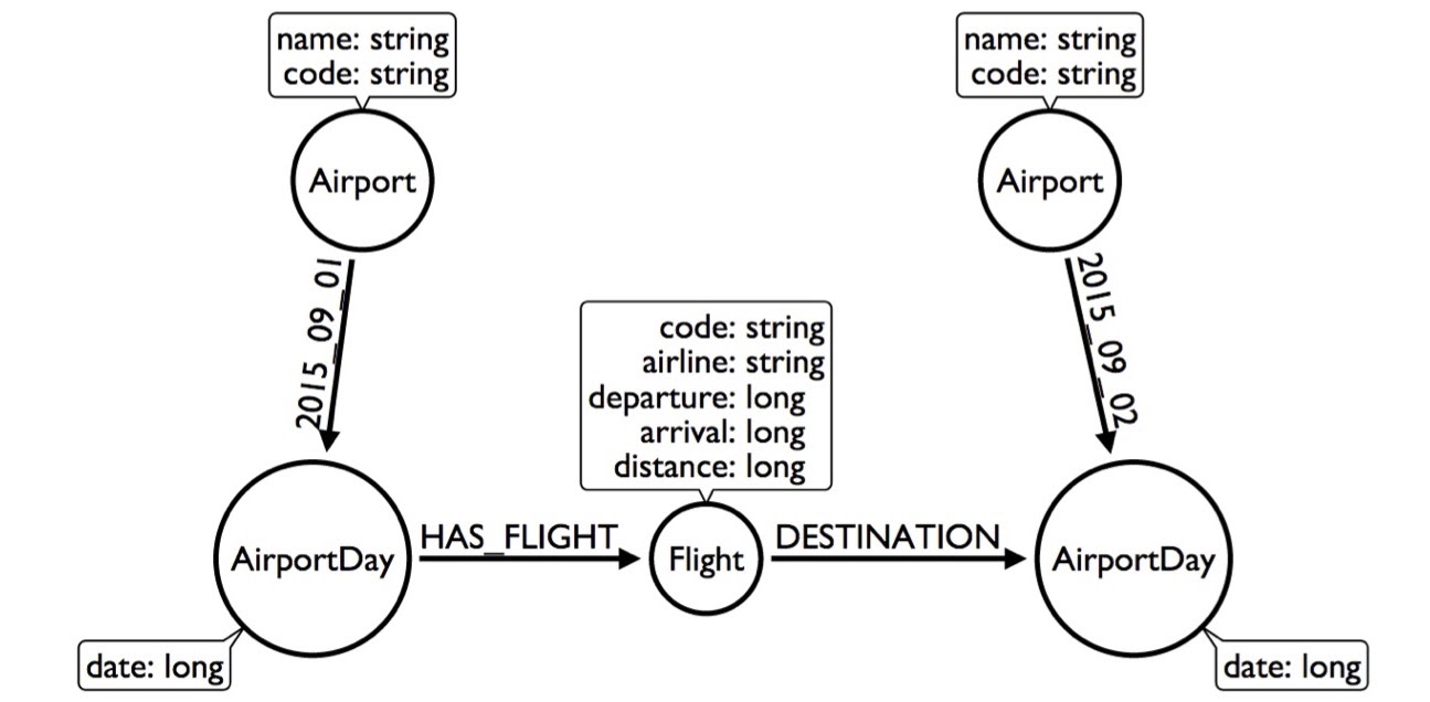
Now we can go from the airport through this dated relationship directly to the airport day. We can even skip looking at the 365 days and go directly, but that doesn’t really buy me much – it only buys me 365 relationships.
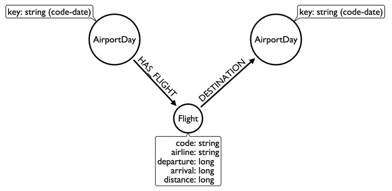
I can make this even faster by getting rid of the airport altogether and labeling the node as code-date, so for every airport, it’ll have many of these airport days:
By now, I’ve already shown you four different ways to model the same data and they’re getting weirder and weirder. Let’s keep going and get a little more creative. Say an AirportDay has 1,000 flights, but only 100 destinations – 20 to Chicago. What we can do is create a Destination node and indicate that this AirportDay has a destination to Chicago. This way, the Destination node would only have 20 flights.
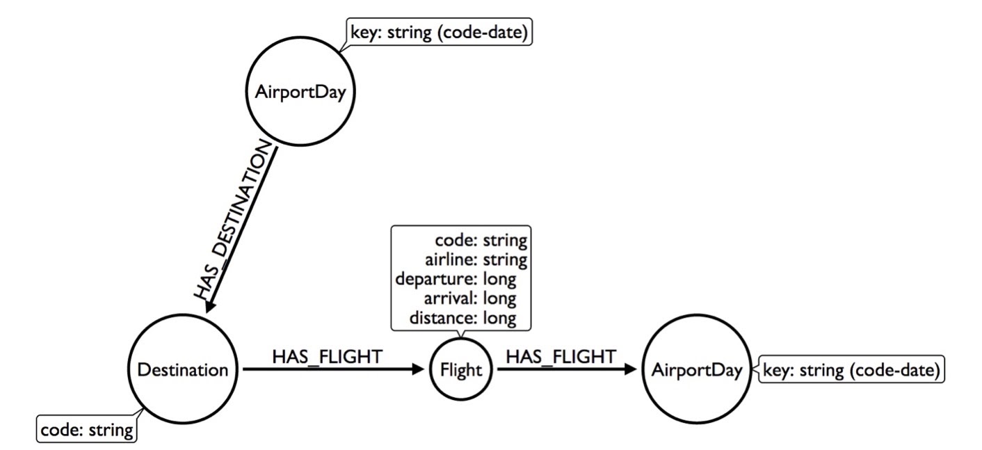
Now I need to look at less of the graph to get the answer, and my query will go faster by creating this Destination node out of thin air.
But I can get even more creative by taking the AirportDay and creating a relationship type that contains the code of the airport. Now this AirportDay will look at the flights going to Chicago, go out that direction, get to the flight and continue on from there.
By using this model, I can skip looking at any flights that go to any destinations that aren’t Chicago. We’re actually promoting a property of the relationship forward so we can skip looking at the part of the graph we don’t really care about.
Why are we doing this? Because every node knows what types of relationships are connected to it, so if we tell it to “go out to the Chicago destination flight relationship,” we can skip everything else. Now, we’re looking at 20 flights, which is going to be incredibly faster than looking at 1,000 flights in a day or 300,000 flights in a year.
The thing to understand here is that there’s no right way to model data in a graph, though there are plenty of wrong ways. You have to get creative and find proper solutions by changing the data a little bit.
If you think this is all insane, take a look at what the folks from Marvel Entertainment have done. In GraphConnect 2013, Peter Olson came along and essentially said: “We have a very complex data model – this is the fantasy world where anything can happen. People go back into the past, into the future and have alternate timelines. How do you model that?” They figured out how to do it in Neo4j using hyperedges. Check it out – it’ll teach you everything you need to know about modeling complex domains. If they can model the fantasy world, you can model the real world.
More modeling: Building a news feed
Let’s talk a little more about modeling, just to drive you guys a little crazy. Say you want to clone Twitter. How would you do something like this in a graph in Neo4j?
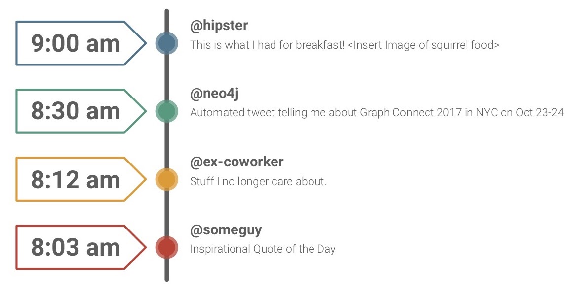
The way it’s done today is that whenever you write a tweet, it’s replicated out to all your followers. Say you have 100 followers – that’s not a big deal. But if you have 10,000,000 followers, it’s a bit of a problem. If you’ve ever tried to edit a tweet, you might’ve realized that you can’t, which is quite weird. That’s the way Twitter was built.
If you were to build a Twitter using a key-value store or object database, you’d do the same. You’d push out these updates into someone’s timeline over and over again; you’ll be basically multiplying your data to all these people. In turn, you’d need to buy lots of servers. That’s not how we work in Neo4j.
Now, you can model the data like this:
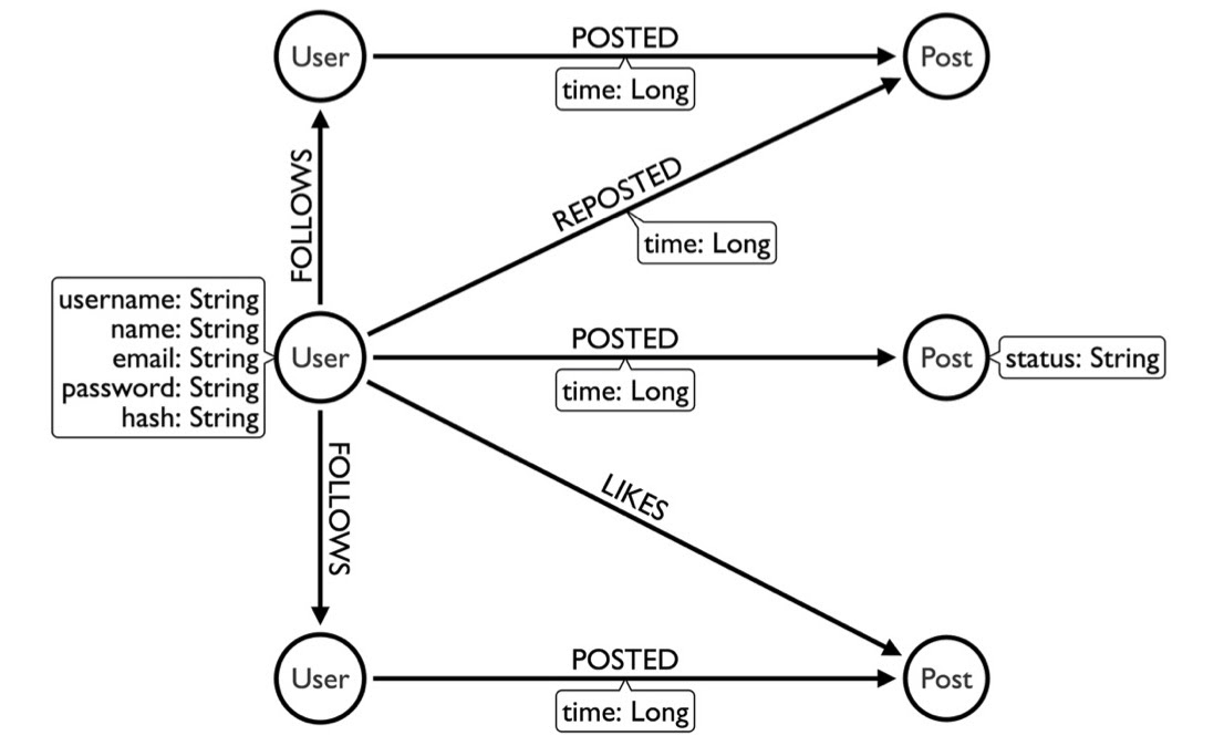
Here, we have a user that follows another user, who posts something. If I wanted to figure out what someone wrote, I can go to the FOLLOWS relationship and see what they’re posting. This post doesn’t need to be duplicated into my timeline; I can just read it (Neo4j is optimized for reads).
The problem with this model is that day one is gonna be fantastic, but on day two, I’m going to have more posts. I’ll need to filter out the posts from yesterday because I only want to see what’s new. And a year from now, I’ll have to filter out all the posts that have been in the last 364 days, because all I want is the new stuff.
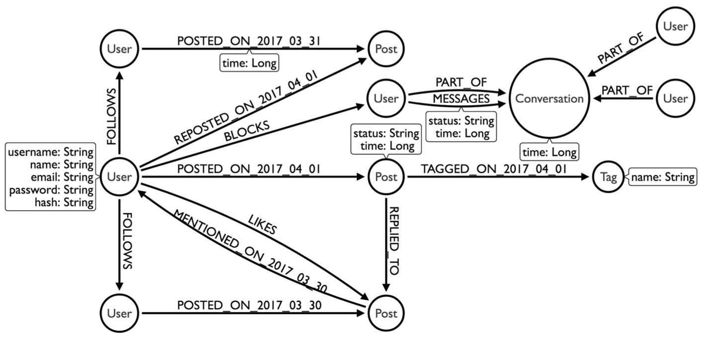
So let’s change the model. Here, we took the date when the post occurred and promoted it as the relationship type:

Now, we can find all the people I follow, see what they posted today or yesterday and do an order-by to sort everything. In this case, my query would only be as big as one day’s worth of postings for the people I follow. It could be one day or five years from now – the query will always take the same amount of time.
And that’s the other trick to Neo4j: if you can write your queries by taking advantage of the data model so that your queries are linear, they’ll scale regardless of how big your data gets. You can expect that same 10 millisecond response time regardless of how big it gets. But, you need to get a little creative in order to make this happen.
Below is the more complex model we came up with. I won’t explain it in-depth, but if you’re really bored, I wrote a 12-part series on how to build a dating site that follows a slightly different model in which people talk to each other and have conversations.
Earlier, I mentioned how every node knows what types of relationships are connected to it, and every node also knows how connected it is to the rest of the graph. The idea is that it knows how many degrees of connections it has; to have a degree of 100, the node knows it has 100 relationships. We can figure this out with the getDegree function:

Moreover, it knows the relationships by type and direction. For example, I can ask how many outgoing friends relationships or incoming likes relationships there are. The nodes know this data because it’s right there in the data model.
Java Core API
Neo4j comes from a Java background and started life as an embedded Java library (The “4j” at the end of Neo4j means Java). If you’re so inclined, you can plug Neo4j as a library into your app and have direct connections to the database. It has an API that you can learn in about a day. You start a transaction, get a node, obtain that node’s properties and traverse the relationship. From there, you either get the properties of the relationship or go to the next node and do it again.
This is what it would look like if you were coding in Java:

As you can see, we start a transaction, find a user and traverse the friends relationship in order to find all the friends of this particular user. Then, we tell it to provide all their properties, throw that into a list and bring it back. It’s fairly easy.
Traversal API
Next, we have the Traversal API, which is insane. I don’t recommend learning this without a few drinks in you. It’s how we used to traverse a graph before we had Cypher, so it’s a little wonky. Really powerful, but takes some getting used to.
We also have bi-directional traversals, which are even worse to wrap your head around, but we have classes for this stuff. It starts off simply by asking, “I want to go with depth-first or breadth-first. I want to go out of these relationships, but not those. For these particular relationships, I want to go in this direction, but not that direction. I want to go no more than five levels deep.”

Whatever you want to do, I can go ahead and write it for you, but you’re better off starting off with something like Cypher, which is easier to learn.
Cypher: Powerful and expressive query language
If you know SQL already, Cypher’s a no-brainer. Most people can look at it even without taking a class and understand what the code is trying to say.
Here’s a person named Dan who loves a person named Ann. We have nodes, relationships and connections.

Below is another, more complex example, with another magic trick, the star *. The star tells the database to keep going. In this example, John Doe is our boss. We want to find John Doe in the graph and see who he manages three levels deep. Let’s look at the Cypher code on the right:

That star means to keep going after three layers deep. You’ll notice a 0 in front of it, which means to include yourself. The boss and everyone he reports to are called a sub; for each sub, you can find out how many people they manage. I’m going to call these guys reports, and I’ll take the count of the reports. This way, I can figure out your whole organization in one tiny query, and if you want to go four, five, 10 layers deep – or however crazy vertically integrated your company is – it doesn’t matter. Just change the number and you’re done.
In contrast, the SQL query on the left is a bit of a mess. Writing that 10-layer-deep query would make you cry.
Cypher stored procedures
For the best of both worlds, mix Cypher and Java. If you’re a Java developer, you can actually take Java, put it into sort procedure, expose it as Cypher and just run the Cypher query:

Use cases
One of the biggest use cases out there is understanding your users, whether you’re looking at building knowledge graphs or using customer 360.
If you want to learn from the experts, there’s a class on YouTube that talks about understanding user behavior by looking at examples such as recommendations and fraud.
So how do you distinguish between what your regular users and not-so-regular users are doing? How do you find suspicious behavior? How do you understand what’s normal and what’s abnormal so we can prevent something bad from happening?
First, you have to understand your users by looking at demographics like age and gender. Let’s say you’re building the next Netflix. Obviously, you’re not going to show every new user the same list of recommended movies. You’ll likely ask a couple of questions, like “what’s your age and gender?” With that, you can provide a more personalized experience.
For example, we know that smaller toddlers might like “Toy Story,” “Toy Story 2” and movies like that. However, men ages 25 to 34 probably enjoy different kinds of movies, such as “Star Wars” and “American Beauty.” Right away, just by knowing your users’ age, you can pick movies out and provide a more fitted experience – at least until you learn more about them. From there, you can drop demographics and look at what individual users are interested in.
Graphs can also be useful for predicting edges. If all these people are connected, they’re likely friends, and you’re probably friends with them too. If your friends – who have similar viewing habits – have watched a particular movie, then you might enjoy the movie too. In this way, you can predict the next edge that’s going to happen in the graph. We can also utilize clustering and community detection algorithms to figure out the groups of users you might have in your system.
Another thing to remember is that recommendations and fraud detection are two sides of the same coin. In a recommendation engine, you’re looking for a relationship that doesn’t exist; you’re trying to predict a new relationship. In fraud detection, you’re doing the opposite; you’re finding a relationship that shouldn’t exist in the graph. For example, if two people are using the same credit card, IP address, device and security number, these are relationships that indicate something’s wrong.
When you’re looking at fraud, you’re modeling user behavior. The obvious fraud sticks out, such as the dot on the top right:

What’s harder to do is finding the fraudsters who pretend to be users, such as the long, vertical line in the center there that feeds into normal user behavior.
Recommendation engines
Let’s quickly build a recommendation engine. Say you’ve watched “Toy Story”; from there, you’re likely going to be recommended “A Bug’s Life.” However, even if you’ve watched “A Bug’s Life,” you would not want to be recommended “The Human Centipede.”
How might we model this? Imagine having a data model that looks like this:

We have a Person who RATED a Movie, and we also have a title and genre for each movie. With this really simple data model, you can build a recommendation model. Here it is in Cypher:
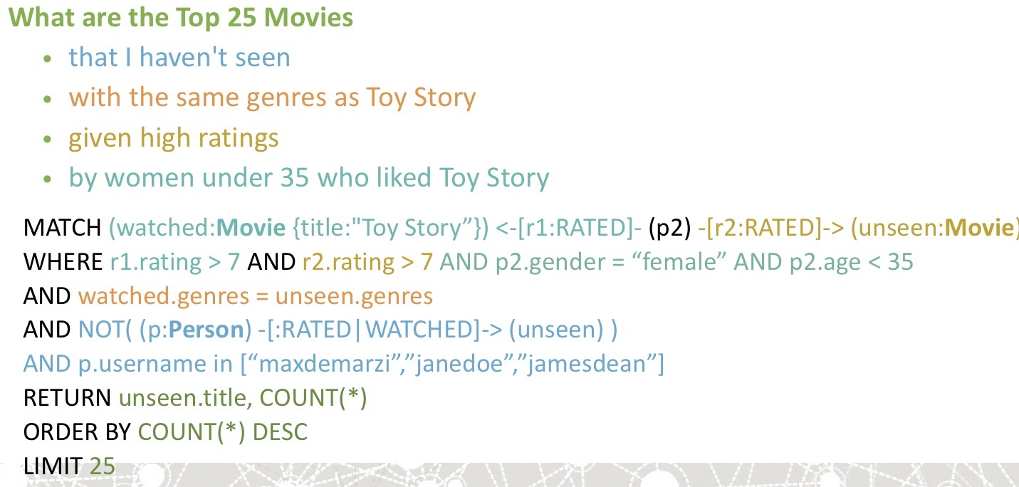
In this scenario, we’re looking for the top 25 movies that I haven’t seen, are in the same genre as “Toy Story” and were also given high ratings by women under 35 who liked “Toy Story.” For this query, we start with the movie “Toy Story,” and we see that p2 is the user who rated this movie. From here, we see the movies they’ve rated (labeling them as unseen), where the rating they gave to “Toy Story” was eight, nine or 10, and the ratings they gave to the unseen movies were also eight, nine or 10. We also want the person’s gender (p2.gender) to be female, and their age to be less than 35 (p2.age < 35). Lastly, we want to make sure that none of the people in this household – maxdemarzi, janedoe and jamesdean – have seen the movie.
As you can see, this is an eight-line recommendation engine that’s looking at user behavior, the characteristics of the movie and the types of the users who are using it for the rating.
You can also build similarity scores for people who have similar viewing habits. We can weigh them highly by saying: “If they watched a movie, you’re probably going to watch what they watched because you exhibit similar behavior.”

This is a crazier query, but it’s still only 10 lines of code if you use k-NN recommendations in Neo4j. First, you find people who are similar to you and then use those people to figure out movies they’ve watched that you haven’t seen yet. Then, we’ll recommend that to you.

Indirect relationships
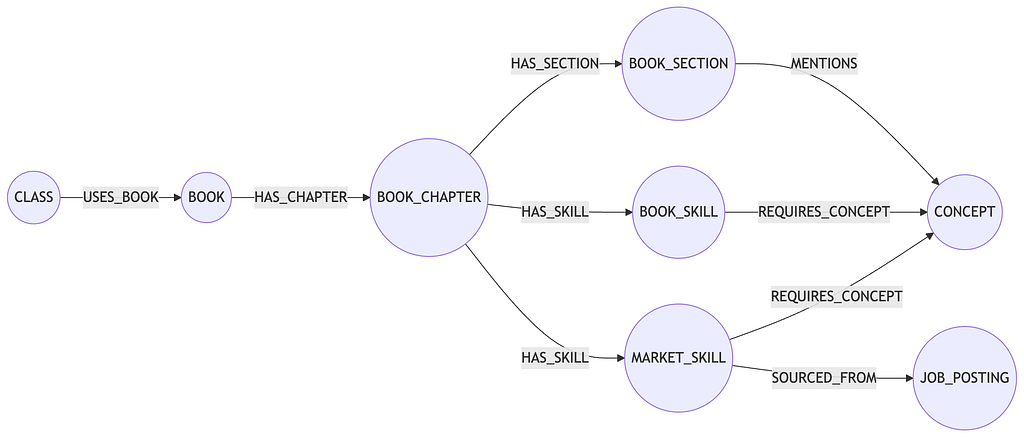
Neo4j is also useful for indirect relationships. For example, we have the following graph, where on one side you have people looking for jobs, and on the other, you have companies looking for people. But, they’re not looking directly for each other; instead, you have a person who lives in a certain location, a job that has some requirements and the candidate who meets those requirements:

Below is your Cypher query. We start off with a user, Max, who lives in a location and has some skills. In that location, there are jobs that require skills that Max also has.

This is a circular match. From here, I can match the skills that the job requires and those that Max also has. With a partial sub-graph match, we can also find the skills that Max does not have, but that the job requires. This gives us a drop-down:

For the first job, you have a 100 percent match – the perfect candidate. But for the second job, you’re missing CSS because nobody puts CSS on their resume anymore. You can just hit the plus button, it’s added to your profile and you match with a second job. However, the third job requires that you know Java. You can click the plus button, lie through your interview and hope for the best.
From the recruiter’s side, they can see all the candidates and choose the best candidate for the position. They can also choose people if no one matches, and thus set a threshold for the requirements needed.
Anyway, there’s a whole bunch of use cases and graph-search you can do. The full presentation is posted online if you’re interested.
Conclusion
The point of the post is to learn the slide below, understand it, sleep with it under your pillow and have it come through your brain.

If you understand this, you’ll also understand Neo4j and why it’s fast. You’ll understand how to model data and write your queries efficiently.
Want to take your Neo4j skills up a notch? Take one of our online training classes or get certified at our GraphAcademy, and level up!
Share Article


Explore
Related Articles
Neo4j Named “One to Watch” in Snowflake’s 2026 Modern Marketing Data Stack Report

Hey LLM, you’re using OPTIONAL MATCH wrong. Here’s the Cypher that actually works.