Graph Algorithms Workflow

How do graph algorithms work?

Graph algorithms run on a graph data model, which is a projection of the stored Neo4j property graph data model. A graph projection can be seen as a view over the stored graph containing only relevant, potentially aggregated, topological, and property information. Graph projections are stored entirely in-memory using compressed data structures optimized for topology and property lookup operations.

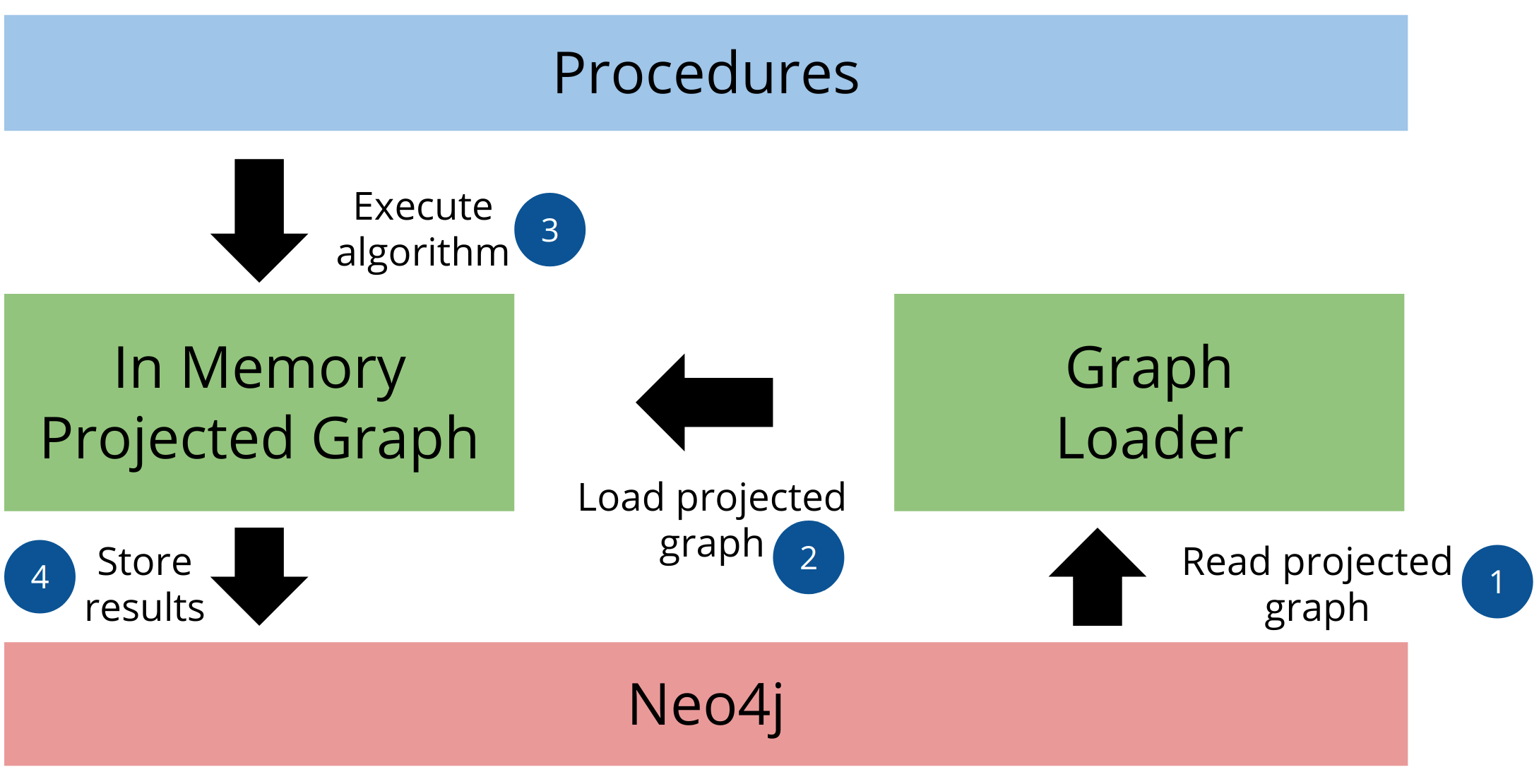
The graph analytics pipeline consists of three main parts. In the first part, the graph loader reads the stored graph from Neo4j and loads it as an in-memory projected graph. You can use either native projection or cypher projection to load the projected graph. In the second step, we execute the graph algorithms on the in-memory projected graph. You can use the results of one graph algorithm as an input to another one. Last but not least, you can stream or store the results back to Neo4j.

Graph management

In this lesson, you will learn the various methods to load an in-memory projected graph which include:

Named graph
Anonymous graph
Native projection
Cypher projection

Named graph

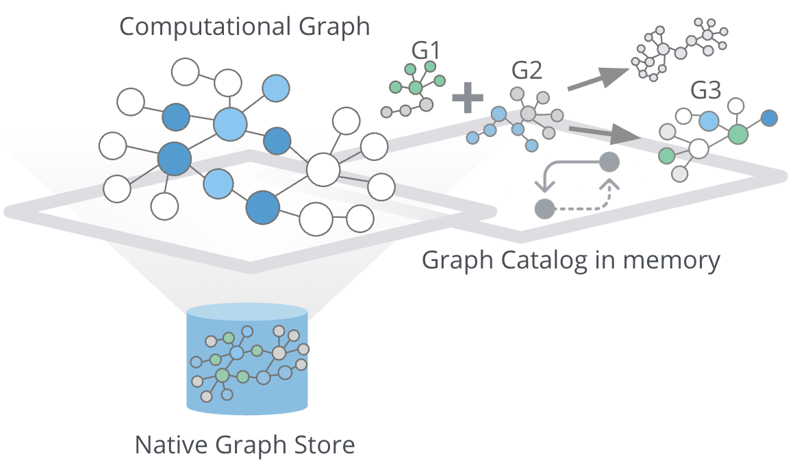
The graph catalog is a concept within the GDS library that allows managing multiple graph projections by name. We call a graph stored in the graph catalog a named graph because you can retrieve it using its name when executing graph algorithms. The advantage of using named graphs is that they can be used many times in the analytical workflow. This way, you do not have to load the projected graph for each algorithm separately, saving time. You can also use the results of one graph algorithm as an input to another graph algorithm. Named graphs can be created using either Native projections or Cypher projections. After usage, named graphs can be removed from the catalog to free up the main memory.

Native projection

A native projection allows you to project a graph from Neo4j into an in-memory graph. The projected graph can be specified in terms of node labels, relationship types, and properties. The main benefit of native projections is their performance. The general syntax for using native projection to load a named graph is:

CALL gds.graph.create(
  <graph-name>, <node-projection>, <relationship-projection>,
    {nodeProperties: String or List,
     relationshipProperties: String or List
     })

With the graph name parameter, you specify the name of the projected graph. The node projection parameter is used to define the nodes you want to project.

Node projection

There are three supported options for the node projection parameter.

String: Used to project a single node label:

'Person'

Using the wildcard operator *, you can project all the node labels in the database.

Array: Used to project multiple node labels:

['Person', 'Organization']

Map: Used for granular node label(s) and property definition:

{
    <node-label>: {
        label: <neo4j-label>,
        properties: {
            <property-key-1>: {
                property: <neo-property-key>,
                defaultValue: <numeric-value>
            },
            <property-key-2>: {
                property: <neo-property-key>,
                defaultValue: <numeric-value>
            }
        }
    }
}

You will very rarely need to use the Map option for the Node projection parameter. If you need to project many labels and their properties, you can use the array input for Node projection combined with the nodeProperties parameter.

Relationship projection

Similarly to Node projection, the Relationship projection also supports three options as an input:

String: Used to project a single relationship type:

'FRIEND'

Using the wildcard operator *, you can project all the relationship types in the database.

Array: Used to project multiple relationship types:

['FRIEND', 'COWORKER']

Map: Used for granular relationship type(s) and property definition:

{
    <relationship-type>: {
        type: <neo4j-type>,
        orientation: <orientation>,
        aggregation: <aggregation-type>,
        properties: <relationship-property-mappings>
    }
}

Orientation

Opposed to Node projection, you use the Map option for projecting relationships more frequently. It allows us to define granular relationship type and properties projection, but has the added orientation and aggregation parameters. The orientation parameter denotes how Neo4j relationships are represented in the projected graph. The following values are allowed:

NATURAL: Each relationship is projected the same way as it is stored in Neo4j (default).
REVERSE: Each relationship is reversed during graph projection.
UNDIRECTED: Each relationship is projected in both natural and reverse orientation.

Multigraph to single graph

The aggregation parameter can be used to reduce a multigraph to a single graph.

Read more about it in the documentation.

Example: Using Native projection

Here is a simple example of using Native projection to project a named graph:

CALL gds.graph.create('graph','Person','HELPS',
    {nodeProperties:['seed'],
     relationshipProperties: ['weight', 'cost']
      })

Here we project a graph consisting of nodes labeled Person and their seed property. In relationship projection, we define a single relationship type HELPS with its weight and cost properties.

Example: More complex projection

Here is a more complex example:

CALL gds.graph.create('graph',
  ['Person', 'Organization'],
  {
  LIKES: {
    orientation: 'UNDIRECTED',
    aggregation: 'DEFAULT',
    type: 'LIKES',
    properties: 'property'
  })

We project a graph that contains nodes labels Person and Organization. For the relationship projection, we use the Map option, where we project the LIKES relationship type with an UNDIRECTED orientation. We did not mention before, but when you load many node labels or relationship types, you can filter them at algorithm execution time. This way, you can, for example, load more relationship types between a single node label and observe how the community structure and node ranking differ between the two networks using a single named graph.

Cypher projection

If the Native projection is not expressive enough to describe the in-memory graph, you can instead use Cypher projection to describe the nodes and relationships. This flexibility is convenient when exploring data and algorithms, and designing a workflow. One benefit of using Cypher projection is the possibility to form a graph from data that exists only at query time. A common use case is the reduction of a 2-hop path to a single relationship. In contrast to Native projection, a Cypher projection is more flexible from the declaration point of view, but less performant. For production, it is recommended to adapt the domain model in a way that it can take advantage of the loading speed of native projections.

The general syntax for using Cypher projection to load a named graph is:

CALL gds.graph.create.cypher(
    '<graph-name>',
    '<node-query>',
    '<relationship-query>'
)

As before, with the graph name parameter, you specify the name of the projected graph. The node query parameter is used to describe the nodes you want to project. The input is a single Cypher query that must return an id of the node. For the id, the Neo4j internal node id is used. Another reserved column is the labels column, which can be used to describe the node’s label. Using the labels column in return allows you to filter node labels at algorithm execution time like with the Native projection.

Example: Preparing for a Relationship projection

Here is an example node query describing all Person and Organization nodes, and returning the internal node id, its label, and the seed property:

MATCH (n) WHERE n:Person OR n:Organization
RETURN id(n) as id, labels(n) as labels, n.seed as seedProperty

The relationship query is used to specify the relationships we want to project. We describe the relationships using the source and target node ids. A reserved column for the relationship type is the type column. It is important to note that the Cypher projection does not support an orientation parameter. Instead, we have to represent an undirected relationship as two directed relationships, where one relationship points in the opposite direction of another.

Example: Preparing for a different Relationship projection

The following relationship query reduces a 2-hop path to a single relationship, effectively representing undirected co-authorship network:

MATCH (p1:Author)-[:WROTE]->(a:Article)<-[:WROTE]-(p2:Author)
RETURN id(p1) AS source, id(p2) AS target, 'COWORKER' as type, count(*) AS weight

Because we use the count() aggregation in the relationship query, we effectively reduce a multigraph to a single graph.

Example: Using the Relationship projections to create the named graph

Putting all this information together, we would use the following syntax to project the undirected coauthorship network:

CALL gds.graph.create.cypher(
    'coauthorship-graph',
    'MATCH (n:Author) RETURN id(n) AS id, labels(n) as labels',
    'MATCH (p1:Author)-[:WROTE]->(a:Article)<-[:WROTE]-(p2:Author)
     RETURN id(p1) AS source, id(p2) AS target, count(a) AS weight'
)

Using Cypher projection

Another example of projecting inferred relationships with Cypher projections is from the Russian Twitter troll analysis.

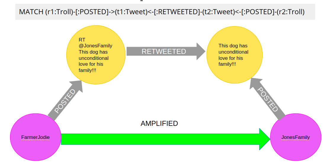
We assume that each re-tweet amplifies the message of the original post by the re-tweeted author. This way, we can find the most influential Twitter users and their community structure in the re-tweet amplification network.

Example: Using Cypher projection

CALL gds.graph.create.cypher(
    'troll-graph',
    'MATCH (n:Troll) RETURN id(n) AS id',
    'MATCH (r1:Troll)-[:POSTED]->(:Tweet)<-[:RETWEETED]-(:Tweet)<-[:POSTED]-(r2:Troll)
     RETURN id(r2) as source, id(r1) as target, count(*) as weight, "AMPLIFIED" as type'
)

Listing all named graphs

If in your analysis you have created named graphs, you can view existing named graphs with the following procedure:

CALL gds.graph.list()

Removing named graphs

After you have finished your graph analysis, you can release the named graph from the main memory.

The syntax to release the named graph from the Graph Catalog is:

CALL gds.graph.drop(<graph-name>)

Anonymous graph

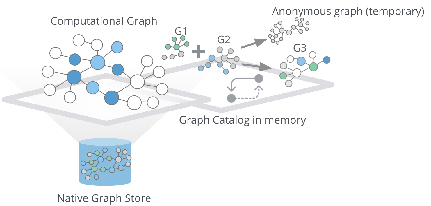
When using the GDSL, the typical workflow is to create a graph and store it in the Graph Catalog. However, if you want to run a single algorithm quickly, it may be convenient to use an anonymous projection. The syntax for describing node labels and relationship types is similar to the ordinary syntax for named graphs. You can use both the Native projection or Cypher projection for describing anonymous graphs.

Native and Cypher projections differ, however, in that relationship projections cannot have more than one property.

Native projection

Instead of separately projecting the in-memory graph, and then later executing a graph algorithm, you describe the Node projection and Relationship projection directly as configuration parameters of an algorithm.

CALL gds.<algo>.<mode>(
  {
    nodeProjection: String, List or Map,
    relationshipProjection: String, List or Map,
    nodeProperties: String, List or Map,
    relationshipProperties: String, List or Map,
    // algorithm and other create configuration
  }
)

Example: Using Native projection with the anonymous graph

Here is an example of executing the PageRank graph algorithm using the anonymous graph with Native projection:

CALL gds.pageRank.stream(
  {
    nodeProjection: 'Person',
    relationshipProjection: ['FRIEND', 'COWORKER'],
    relationshipProperties: 'weight',
    relationshipWeightProperty:'weight'
  }
)

Cypher projection

Similarly to using Native projection on an anonymous graph, you can describe the Node query and Relationship query directly as configuration parameters of an algorithm:

CALL gds.<algo>.<mode>(
  {
    nodeQuery: Cypher Query,
    relationshipQuery: Cypher Query,
    // algorithm and other create configuration
  }
)

Example: Using Cypher projection with the anonymous graph

Here is an example of executing the PageRank graph algorithm using the anonymous graph with Cypher projection:

CALL gds.pageRank.stream(
  {
    nodeQuery: 'MATCH (n:Author) RETURN id(n) AS id',
    relationshipQuery: 'MATCH (p1:Author)-[:WROTE]->(a:Article)<-[:WROTE]-(p2:Author)
                        RETURN id(p1) AS source, id(p2) AS target, count(a) AS weight',
    relationshipWeightProperty:'weight'
  }
)

How to use graph algorithms

All product-supported graph algorithms feature four modes of execution:

Stream
Stats
Write
Mutate

Stream mode

The stream mode will return the results of the algorithm computation as Cypher result rows. This is similar to how standard Cypher queries operate.

The returned data can be a node id and a computed value for the node (such as a Page Rank score, or WCC componentId), or two node ids and a computed value for the node pair (such as a Node Similarity similarity score).

If the graph is very large, the result of a stream mode computation will also be very large. Using the ORDER BY and LIMIT clauses in the Cypher query could be useful to support 'top N'-style use-cases.

The general syntax to use the stream mode is:

CALL gds.<algo>.stream()

Stats mode

The stats mode returns statistical results for the algorithm computation like counts or percentile distributions. A statistical summary of the computation is returned as a single Cypher result row.

The direct results of the algorithm are not available when using the stats mode. This mode forms the basis of the mutate and write execution modes, but does not attempt to make any modifications or updates anywhere.

The general syntax to use the stats mode is:

CALL gds.<algo>.stats()

Write mode

The write mode will write the results of the algorithm computation back to the Neo4j database. This is similar to how standard Cypher writing queries operate.

A statistical summary of the computation is returned, similar to the stats mode. This is the only execution mode that will attempt to make modifications to the Neo4j database.

The written data can be node properties (such as Page Rank scores), new relationships (such as Node Similarity similarities), or relationship properties. The write mode can be very useful for use-cases where the algorithm results would be inspected multiple times by separate queries since the computational results are handled entirely by the library.

For the results from a write mode computation to be used by another algorithm, a new graph must be created from the Neo4j database with the updated graph.

The general syntax to use the write mode is:

CALL gds.<algo>.write()

Mutate mode

The mutate mode will write the results of the algorithm computation back to the in-memory graph.

Note that the specified mutateProperty value must not exist in the in-memory graph beforehand. This enables running multiple algorithms on the same in-memory graph without writing results to Neo4j in-between algorithm executions.

This execution mode is especially useful in three scenarios:

Algorithms can depend on the results of previous algorithms without the need to write to Neo4j.
Algorithm results can be written together (see write node properties and write relationships).
Algorithm results can be queried via Cypher without the need to write to Neo4j at all (see gds.util.nodeProperty).

A statistical summary of the computation is returned similar to the stats mode. Mutated data can be node properties (such as Page Rank scores), new relationships (such as Node Similarity similarities), or relationship properties.

The general syntax to use the mutate mode is:

CALL gds.<algo>.mutate()

Guided Exercise: Getting started with the graph algorithms workflow

Follow along with this video to become familiar with the GDSL Graph Management in Neo4j NEuler.

Exercise: Graph algorithms workflow

In NEuler: Run the Degree centrality algorithm on the Character labels and INTERACTS_SEASON1 relationship types and observe the generated code to run the algorithms using anonymous or named graphs.
In Neo4j Browser: :play 4.0-intro-graph-algos-exercises and follow the instructions for Graph Catalog.

Estimated time to complete: 20 minutes

Summary

In this lesson, you learned some best practices for working with graph algorithms as part of your analytics workflow.

Check Answers

Need help? Ask in the Neo4j Community

Graph Algorithms Workflow

How do graph algorithms work?

Graph management

Named graph

Native projection

Node projection

Relationship projection

Orientation

Multigraph to single graph

Example: Using Native projection

Example: More complex projection

Cypher projection

Example: Preparing for a Relationship projection

Example: Preparing for a different Relationship projection

Example: Using the Relationship projections to create the named graph

Using Cypher projection

Example: Using Cypher projection

Listing all named graphs

Removing named graphs

Anonymous graph

Native projection

Example: Using Native projection with the anonymous graph

Cypher projection

Example: Using Cypher projection with the anonymous graph

How to use graph algorithms

Stream mode

Stats mode

Write mode

Mutate mode

Guided Exercise: Getting started with the graph algorithms workflow

Exercise: Graph algorithms workflow

Check your understanding

Question 1

Question 2

Question 3

Summary