Massive Parallel Imports in Neo4j Without Deadlock and Lock Contention

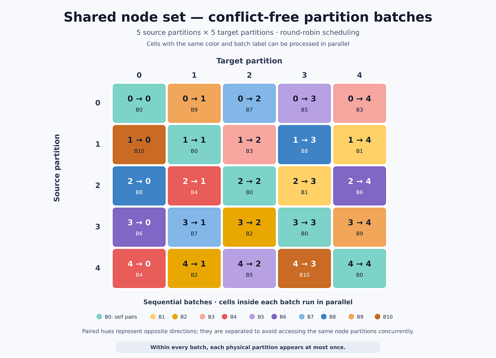
Optimizing graph import partitioning based on workers and k-1 coloring algorithm.

This article is a generalization of the approach designed by Eric MONK in his article “Mix and batch: a technique for fast, parallel relationship loading in Neo4j”. It explains the theoretical underpinnings and ideas. A follow up article will show the practical application and provide the source code repository.

Mix and batch: a technique for fast, parallel relationship loading in Neo4j – Neo4j Graph Intelligence Platform

His approach uses the final digits of source and target node IDs to build non-overlapping partitions, then groups the resulting matrix cells along cyclic diagonals into sequential batches that can be loaded in parallel without accessing the same node sets concurrently. The approach has two main limitations:

1. Deriving partitions from the final digits of node IDs does not adapt the partition count to the available workers;
2. Diagonal batching is unsafe when source and target nodes are not disjoint (for example, if you create relationships between Person nodes).

That’s why we propose the following improvements to overcome the previous limits:

• Compute partitions based on the number of workers using a hash function;
• A new function to import relationships where source and target nodes are from the same set (meaning they are not disjoint);
• Use the K-1 coloring algorithm to compute batches of partitions that can be imported in parallel.

Compute partitions

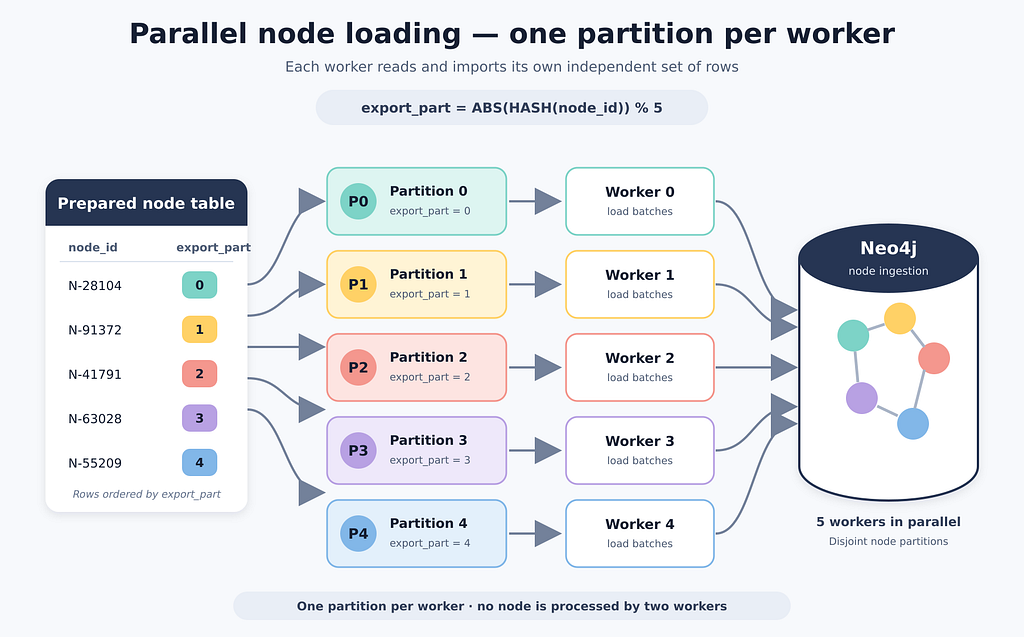
Generally, when data is loaded in batches, there is one table for nodes and one table for relationships. This step consists of calculating a new column (called export_part) for these tables.

Instead of using the last part of the node identifier, as in the original article, you can use an elegant method proposed by Mathieu EPLENIER, in which partitions of your source tables are computed using the formula below.

For an optimal import, partition_count is equal to the number of workers of the server allocated to the data import. This provides enough independent work to feed the worker pool without hard-coding partition boundaries in the source data.

For nodes

export_part = HASH(id) modulo partition_count

The SQL expression in Snowflake becomes:

CAST(
    ABS(HASH(node_id)) % partition_count
    AS VARCHAR
) AS export_part

If partition_count = 5, the node table contains up to 5partition values, from 0to 4.

For relationships

source_partition = HASH(id_source) modulo partition_count
target_partition = HASH(id_target) modulo partition_count
export_part = source_partition + " - " + target_partition

The SQL expression in Snowflake becomes:

CAST(
    ABS(HASH(id_source)) % partition_count
    AS VARCHAR
)
|| ' - ' ||
CAST(
    ABS(HASH(id_target)) % partition_count
    AS VARCHAR
) AS export_part

If partition_count = 5, the relationship table contains up to 5²=25 partition values, from 0 – 0 to 4 – 4.

This method is deterministic and guarantees that you to have disjoint partitions. However, this does not guarantee that the partitions will be the same size, as this depends on the data structure.

Now, it is necessary to answer the question: which partition can we import in parallel?

Import nodes

For the node tables, it’s trivial because it will load one partition per worker. Therefore, all partitions will be imported simultaneously.

Import relationships

For relationship tables, it’s a bit more complex because it depends on whether the source and target nodes are disjoint or non-disjoint.

To do this, we need to construct a square matrix of size equal to the number of partitions; in our example, it is 5.

This will allow us to know which partitions can be imported in parallel and maximize the use of workers.

Between disjoint nodes

The diagonal method used in “Mix and batch: a technique for fast, parallel relationship loading in Neo4j” works well when the source and target nodes are not in the same set. Indeed, after computing the partitions, we can create a matrix in which each cell contains a partition. Each diagonal of the matrix corresponds to a batch of partitions that can be loaded in parallel.

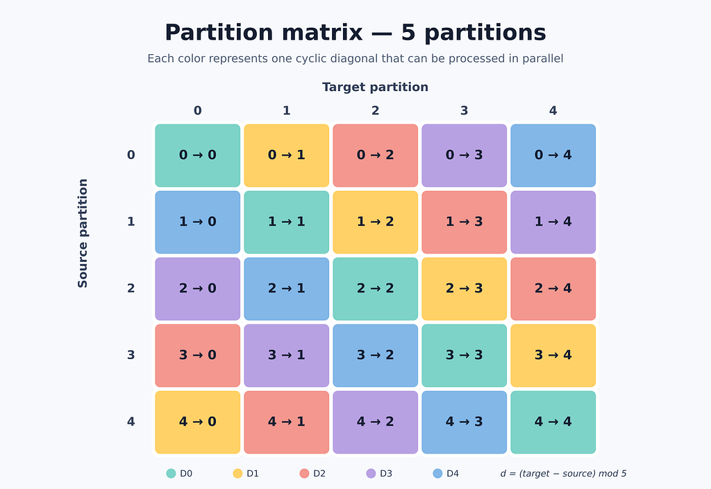
Each color represents a batch containing partitions that can be imported in parallel without deadlock and lock contention.

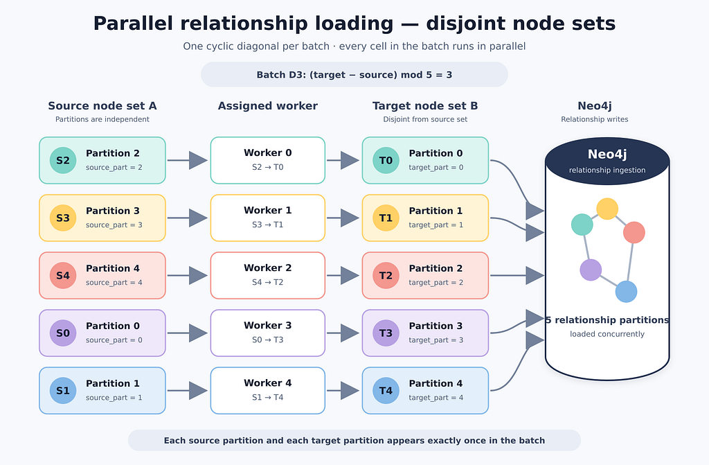
For example, D3 partitions can be imported in parallel without deadlock or lock contention, as illustrated in the following image:

Python code

def diagonals(partition_count: int) -> list[list[str]]:
    """Return parallel batches (cyclic diagonals) from a source-target partition matrix.
    
    The source and target node sets are disjoint, and each set is divided
    into ``partition_count`` partitions. Their combinations form a square
    matrix containing ``partition_count ** 2`` source-target partition pairs.

    The function divides this matrix into ``partition_count`` cyclic
    diagonals. Each cyclic diagonal represents a batch of partitions that can be
    processed in parallel. Within a batch, every source partition and every
    target partition appears exactly once, preventing concurrent tasks from
    accessing the same partition.

    Args:
        partition_count: Number of partitions in each node set.

    Returns:
        A list of parallel batches. Each batch represents a cyclic diagonal
        and contains partition pairs in ``"source - target"`` format.
    """
    return [
        [
            f"{(diagonal_index + target_partition) % partition_count}"
            f" - {target_partition}"
            for target_partition in range(partition_count)
        ]
        for diagonal_index in range(partition_count)
    ]

Between non-disjoint nodes

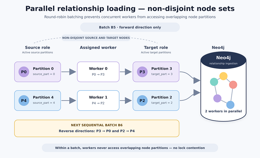
However, if you want to import relationships between nodes coming from the same set, then you will get deadlock errors. That’s why we need another function defined below to handle this case using round-robin rotation.

Here too, each color represents a batch of partitions that can be imported in parallel without deadlocks or lock contention. The only difference lies in the reduced number of partitions per batch, which implies fewer processing steps than for batches generated by the diagonal function.

For example, B5 partitions can be imported in parallel without deadlock or lock contention, as illustrated in the following image:

Python code

def relationship_batches(partition_count: int) -> list[list[str]]:
    """Return parallel batches for a non-disjoint partition matrix.

    The source and target nodes belong to the same node set, which is divided
    into ``partition_count`` partitions. Their combinations form a square
    matrix containing ``partition_count ** 2`` source-target partition pairs.

    Each batch contains pairs that do not share any partition. Therefore, all
    pairs in the same batch can be processed in parallel without concurrently
    accessing the same node partition.

    The batches are generated using a round-robin rotation. Forward and reverse
    pairs are placed in separate batches because they access the same
    partitions.

    Args:
        partition_count: Number of partitions in the node set.

    Returns:
        A list of parallel batches containing partition pairs in
        ``"source - target"`` format.
    """
    # Self-referencing pairs use distinct partitions and can therefore be
    # processed together.
    batches = [
        [
            f"{partition} - {partition}"
            for partition in range(partition_count)
        ]
    ]

    partitions = list(range(partition_count))

    # Round-robin pairing requires an even number of values. For an odd number
    # of partitions, None represents the partition that rests during a round.
    if partition_count % 2:
        partitions.append(None)

    # Keep one partition fixed while rotating all the others around it.
    # The fixed partition acts as an anchor and prevents the rotations from
    # generating the same pairs repeatedly.
    fixed_partition = partitions[0]
    rotating_partitions = partitions[1:]

    # Keeping one value fixed and rotating the remaining values generates
    # every possible unordered partition pair exactly once.
    for _ in range(len(partitions) - 1):
        current_partitions = [
            fixed_partition,
            # Unpack the rotating partitions to form the current round of pairs.
            *rotating_partitions
        ]

        # Pair values placed at opposite positions in the current round.
        # Each real partition can appear in at most one pair.
        pairs = [
            (current_partitions[index], current_partitions[-1 - index])
            for index in range(len(current_partitions) // 2)
            if current_partitions[index] is not None
            and current_partitions[-1 - index] is not None
        ]

        # Forward pairs do not share any physical partition and can therefore
        # be processed in parallel.
        batches.append([
            f"{source_partition} - {target_partition}"
            for source_partition, target_partition in pairs
        ])

        # Reverse pairs must be placed in a separate batch because they use
        # the same physical partitions as their corresponding forward pairs.
        batches.append([
            f"{target_partition} - {source_partition}"
            for source_partition, target_partition in pairs
        ])

        # Rotate every partition except the fixed anchor. The last rotating
        # partition moves to the front for the next round.
        rotating_partitions = [
            rotating_partitions[-1],
            *rotating_partitions[:-1],
        ]

    return batches

Thus, importing relationships in batches using partitions calculated by these functions helps to avoid deadlocks and lock contention.

Generic function using the K-1 Coloring algorithm

Previously, we used two Python functions to determine which partitions could be imported in parallel. They were designed to compute optimal partition batches from a matrix (since a relationship is created between two nodes). Now, imagine you need to compute partition batches from a more complex graph, such as a simplicial complex. It’s a high-level graph where relationships can connect x nodes.

This is where you can use the K-1 Coloring algorithm from the Neo4j Graph Data Science library to compute batches of partitions. We model each source-target partition pair as a node and connect two nodes when their relationship loads at least one common node partition. K-1 coloring assigns different colors to the adjacent nodes, allowing each color group to form a conflict-free parallel batch (provided the algorithm has converged), while the different color groups are processed sequentially.

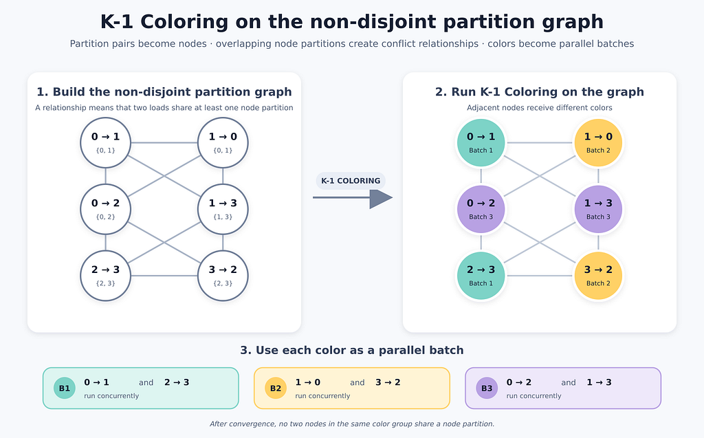
Since the algorithm is not deterministic, you will have a working solution, but it won’t be optimal (in terms of speed in our context).

To illustrate this, the following Cypher queries create the previous matrix of partitions and apply the K-1 Coloring algorithm to compute batches of partitions.

Cleanup queries

// Drop relationships
MATCH ()-[r:SHARES_PARTITION_NOT_DISJOINT|SHARES_PARTITION_DISJOINT]->()
CALL (r){
    DELETE r
} IN TRANSACTIONS OF 1000 ROWS
FINISH;

// Drop nodes
MATCH (n:Partition)
CALL (n) {
    DELETE n
} IN TRANSACTIONS OF 1000 ROWS
FINISH;

Graph creation

// Set grid parameter
:param grid => 5;

// Query to create nodes grid
WITH $grid AS grid
UNWIND range(0, grid - 1) AS sourcePartition
UNWIND range(0, grid - 1) AS targetPartition
CALL (grid, sourcePartition, targetPartition) {
    MERGE (p:Partition {
        grid: grid
        , id: toString(sourcePartition) + "-" + toString(targetPartition)
    })
    SET p.sourcePartition = sourcePartition
        , p.targetPartition = targetPartition
}
FINISH;

// Query to create relationships between partitions
MATCH (a:Partition {grid: $grid})
MATCH (b:Partition {grid: $grid})
WHERE a < b
CALL (a, b) {
    // When the nodes are not disjoint (The source and target nodes belong to the same set)
    WITH a, b
    WHERE a.sourcePartition = b.sourcePartition
    OR a.sourcePartition = b.targetPartition
    OR a.targetPartition = b.sourcePartition
    OR a.targetPartition = b.targetPartition
    MERGE (a)-[r:SHARES_PARTITION_NOT_DISJOINT]->(b)
    UNION
    // When the nodes are disjoint (The source and target nodes belong to different sets)
    WITH a, b
    WHERE a.sourcePartition = b.sourcePartition
    OR a.targetPartition = b.targetPartition
    MERGE (a)-[r:SHARES_PARTITION_DISJOINT]->(b)
}
FINISH;

Running K-1 Coloring

// GDS projection
CYPHER runtime=parallel
// SHARES_PARTITION_NOT_DISJOINT OR SHARES_PARTITION_DISJOINT
MATCH (source)-[r:SHARES_PARTITION_NOT_DISJOINT]->(target)
RETURN gds.graph.project(
    'grid'
    , source
    , target
    , {}
    , { undirectedRelationshipTypes: ['*'] }
) AS graph;

// Run K-1 Coloring algorithm (stream mode)
CALL gds.k1coloring.stream('grid', {maxIterations: 100, concurrency: 4})
YIELD nodeId, color
RETURN color, collect(gds.util.asNode(nodeId).id) AS partitions;

// Drop in-memory graph projection
CALL gds.graph.drop('grid', false)
YIELD graphName
RETURN graphName;

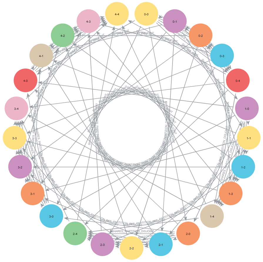
Resulting batches when the nodes are disjoint (table and graph view):

╒═════╤═══════════════════════════════════╕
│color│partitions                         │
╞═════╪═══════════════════════════════════╡
│0    │["0-0", "1-1", "2-2", "3-3", "4-4"]│
├─────┼───────────────────────────────────┤
│1    │["0-1", "1-0", "3-2", "2-3"]       │
├─────┼───────────────────────────────────┤
│2    │["0-2", "2-0", "3-1", "1-3"]       │
├─────┼───────────────────────────────────┤
│3    │["0-3", "3-0", "2-1", "1-2"]       │
├─────┼───────────────────────────────────┤
│4    │["0-4", "4-0"]                     │
├─────┼───────────────────────────────────┤
│5    │["4-1", "1-4"]                     │
├─────┼───────────────────────────────────┤
│6    │["4-2", "2-4"]                     │
├─────┼───────────────────────────────────┤
│7    │["4-3", "3-4"]                     │
└─────┴───────────────────────────────────┘

Resulting batches when the nodes are not disjoint (table and graph view):

╒═════╤═══════════════════════════════════╕
│color│partitions                         │
╞═════╪═══════════════════════════════════╡
│0    │["0-0", "1-1", "2-2", "3-3", "4-4"]│
├─────┼───────────────────────────────────┤
│1    │["0-1", "2-3"]                     │
├─────┼───────────────────────────────────┤
│2    │["0-2", "1-3"]                     │
├─────┼───────────────────────────────────┤
│3    │["0-3", "1-2"]                     │
├─────┼───────────────────────────────────┤
│4    │["0-4", "2-1"]                     │
├─────┼───────────────────────────────────┤
│5    │["1-0", "2-4"]                     │
├─────┼───────────────────────────────────┤
│6    │["2-0", "1-4"]                     │
├─────┼───────────────────────────────────┤
│7    │["3-0", "4-1"]                     │
├─────┼───────────────────────────────────┤
│8    │["4-0", "3-1"]                     │
├─────┼───────────────────────────────────┤
│9    │["3-2"]                            │
├─────┼───────────────────────────────────┤
│10   │["4-2"]                            │
├─────┼───────────────────────────────────┤
│11   │["3-4"]                            │
├─────┼───────────────────────────────────┤
│12   │["4-3"]                            │
└─────┴───────────────────────────────────┘

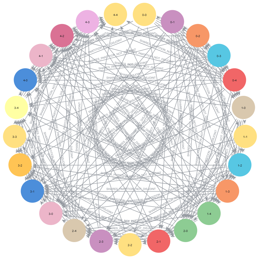
As you can see, the solutions provided by K-1 Coloring are not as optimal as those from the Python functions. However, this offers an effective alternative in complex parallelization cases.

Each color represents a batch of partitions that can be imported in parallel. For example, with color 2, one worker will import relationships where the partition is0 – 2 while another worker will import relationships where the partition is 4 – 4 .

Conclusion

In conclusion, this article proposes a generic and optimal solution for partitioning your data tables (representing nodes and relationships) and then calculating batches of partitions that can be imported into Neo4j in parallel without deadlocks or lock contention.

This article applies to cases where nodes and relationships are imported in batches using any drivers.

Enjoy a world free from deadlock and lock contention during your import!

---

Massive Parallel Imports in Neo4j Without Deadlock and Lock Contention was originally published in Neo4j Developer Blog on Medium, where people are continuing the conversation by highlighting and responding to this story.