Understanding GraphSAGE

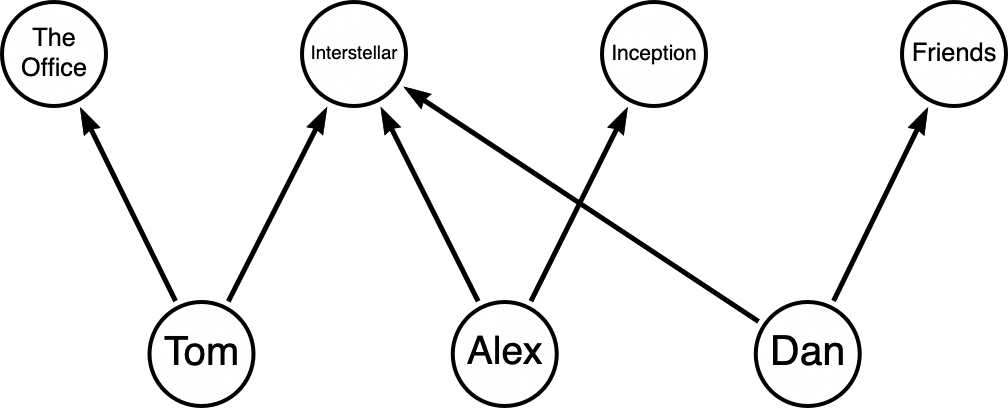
Consider the graph below, which models a movie content platform. You have various users and a few movies and TV shows that users have watched. To keep things simple, there will be only four programs and three users. If you wanted to compare different movies to each other, you might want to consider embeddings. Embeddings can transform a graph structure into a vector of numbers, which can be used in downstream machine learning tasks.

Turning Graph Features into a Numeric Vector

GraphSAGE is an inductive embedding model. That means you can generate embeddings for new nodes without having to retrain on your whole graph. It works in three (mostly) simple steps:

1. Take a uniform sample from the neighborhood of a node
2. Aggregate embeddings from those sampled neighbors
3. Find the correct weights and bias to either predict a supervised target or to match the graph structure

The core of the method is captured in the algorithm below:

embedding = activation(W * AVG[own_feature, neighbor_summary] + b)

GraphSAGE will multiply both a node’s own features and the features of its neighbors by learned weights to get a set of embeddings. Those embeddings will be compared to either a target value (in supervised mode) or to a connected node’s embeddings to measure error. Finally, using gradient descent, GraphSAGE will seek to find a set of weights that minimizes this error.

Capturing a node’s and its neighbor’s features

Sampling Neighbors

First, you need to take a uniform sample of neighbors. You get to choose how many neighbors will be in your sample. In this case, our sample will consist of two neighbors for a given node. So, if you wanted to create embeddings for each movie in your graph, you might take a sample of two neighbors from each movie. So in the case of Interstellar, that will be Alex and Dan. And in the case of “The Office”, which only has one neighbor, you will take Tom twice.

Aggregate Feature Information from Neighbors

Now, let’s say that each user in our graph has some simple features, such as preference scores for different genres:

• Alex: Sci-Fi score = 9 (loves sci-fi)
• Dan: Sci-Fi score = 3 (not really into it)
• Tom: Sci-Fi score = 7

The simplest way to aggregate features belonging to your sample of neighbors would be just to average them together across the sample. So for Interstellar’s case, that would be (9 + 3)/2 or 6. And for The Office, that would be (7+7)/2 or 7.

These single numbers are neighbor summaries for each movie. Before you move on, some things are worth knowing:

• Mean is just the simplest option – the original GraphSAGE paper also proposes fancier aggregators, like feeding the neighbors through a small neural network first
• Order shouldn’t matter – neighbors do not have a natural order to them, so whatever method you use to aggregate them should result in the same value, no matter what aggregation function you choose
• Features will be stored in vectors – typically, you will be aggregating multiple different features and compressing them down into a vector. So there might be preferences for different genres beyond just science fiction

Combine your own features with the neighbor summary

Every movie will also have its own features. In this example, each movie has a thumbs-up percentage:

• Interstellar: 92% thumbs up
• The Office: 88% thumbs up
• Inception: 95% thumbs up
• Friends: 85% thumbs up

So let’s zoom back into Interstellar and your efforts to turn it into an embedding. We will hold these different measures together as a vector:

[92, 6]

This combined vector gets passed through a small neural network layer, which is basically a weighted combination followed by a squashing function, to produce Interstellar’s brand new embedding. Roughly:

embedding = activation(W * [92, 6] + b)

Where:

• W (weights) and b (bias) are the numbers the model learns during training. They decide how much to trust “thumbs up percent” vs “neighbor sci-fi score” when forming the final embedding
• Activation is the squashing function (commonly ReLU) that keeps the output well-behaved

The key idea here is that the model actually learns how to weigh these two pieces. If it turns out that “who watches” is a stronger recommendation signal than “raw thumbs up score,” then the training will push W to lean more heavily on the neighbor-summary side and vice versa.

Determining Weights and Bias – Supervised Version

The beauty of GraphSAGE is that it can create either supervised or unsupervised embeddings. Supervised learning means the model learns from labeled examples. You tell it the right answer during training, so it learns to predict that answer on new data. Unsupervised learning means there are no labels. The model just finds patterns or structure in the data on its own. In GraphSAGE, that translates to: supervised = train embeddings to predict a known target (like a particular node property), unsupervised = train embeddings just from the graph’s connectivity.

You can create a simple label indicating whether a movie is considered a hit, and GraphSAGE will try to optimize its weights and bias to match those labels. If a movie has more than 90% thumbs-up, it is considered a hit. If not, it’s a miss.

• Interstellar: 92% = Hit
• Inception: 95% = Hit
• The Office: 88% = Miss
• Friends: 85% = Miss

So if a hit is anything with a rating above 90%, can you predict what would be a hit? In our incredibly simple example, you only have two features to work with, and one of them was used to derive the label. So the only input to our model is the neighbor summary.

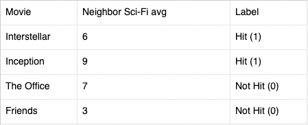
Here, you will do a classic pattern in machine learning, guess and check. GraphSAGE will make a prediction using weight and bias, then compare it against the actual recorded score. The gap between the predicted and actual values is the error or loss.

Our starting random weights will be: W = 0.1 and b = 0, therefore:

prediction = sigmoid(W × 6 + b) = sigmoid(0.6) ≈ 0.65

Note: the sigmoid here simply ensures the result is between 0 and 1

But the true label is 1, whereas the predicted probability was 0.65. That prediction was too low, so the error tells us: “push W and b up a bit, so your input produces a high output next time.” You then do this for every node in the graph, and gradient descent finds the balance that gets predictions closest to all four true labels at once. Repeat this process over many passes, and W and b settle into good values.

Determining Weight and Biases – Unsupervised Edition

Unlike the supervised version, you don’t need a derived label such as “Hit” or “Miss” here. The rule is actually simpler: nodes that are connected in the graph should have similar embeddings, and nodes that aren’t connected should have dissimilar embeddings. Let’s consider Alex for this example:

• Alex watched Interstellar
• Alex did not watch Friends

Step 1: Create embeddings from random weights

Just like before, we will start with random weights, say w =[0.1, 0.1], b = 0. Passing Alex, Interstellar, and Friends through the formula below will give you some pretty meaningless results:

embedding = activation(W * AVG[own_feature, neighbor_summary] + b)

• Alex: 0.5
• Interstellar: 0.4
• Friends: 0.9

Step 2: Measure Similarity

A common way to measure how similar two embeddings are is the dot product, where you simply multiply the two values together (note: with real vectors, you’d multiply matching positions and add them up, but since we’re using single numbers, it’s just multiplication):

Alex · Interstellar = 0.5 × 0.4 = 0.20

Alex · Friends = 0.5 × 0.9 = 0.45

Notice the issue? Since Alex watched Interstellar, you want that similarity score to be high, and vice versa for friends. This mismatch is the error signal that GraphSAGE will correct for.

Step 3: Adjust W and b to fix it

Gradient descent nudges the weights so that, next time around, Alex’s and Interstellar’s embeddings get pulled closer together (raising that dot product), while Alex’s and Friends’ embeddings get pushed further apart (lowering it). Repeat this across every real edge and made-up non-edge in the graph thousands of times, and the weights gradually settle into values where “connected in the graph” reliably means “similar embedding,” with no labels required anywhere.

Second Hop Embeddings

So far, everything you have looked at has been about a node’s direct neighbors. But typically, GraphSAGE will go further by stacking multiple layers. This lets information travel two, three, or even more hops across the graph. Each layer will have its own weights and biases.

Alex and Tom are not directly connected in the graph, but both watched Interstellar, and you want your final embeddings to reflect that shared connection. So how does GraphSAGE bake that friend-of-friend connection into the embeddings it generates?

Step 0: Interstellar’s 1 Hop Embedding

First return to calculating the embedding for Interstellar. Earlier, you learned how such an embedding might be calculated, but you never arrived at specific weights and biases. So let’s just say that the training converged with a plausible score like W = [0.4, 0.9], b = 0.2. There are two weights because Interstellar’s embedding captures two features: the thumbs-up and its neighbor summary. So if you wanted to calculate the embedding for Interstellar, that would be:

h¹(Interstellar) = ReLU(0.4×92 + 0.9×6 + 0.2) = ReLU(36.8 + 5.4 + 0.2) = ReLU(42.4) = 42.4

Step 1: Find the Embeddings of Interstellar’s Direct Neighbors

Both Alex and Dan watched Interstellar. So you will need to have their embeddings.

For Alex, you have two features: his Sci-Fi score (9) and his neighbor summary (93.5), which yields the following embedding:

h¹(Alex) = ReLU(0.4×9 + 0.9×93.5 + 0.2) = ReLU(3.6 + 84.15 + 0.2) = ReLU(87.95) = 87.95

Dan is much the same. He has two neighbors because he watched Inception and Friends, giving him a neighbor summary of 90, and his Sci-Fi score = 3. Therefore, his embedding will be:

h¹(Dan) = ReLU(0.4×3 + 0.9×90 + 0.2) = ReLU(1.2 + 81 + 0.2) = ReLU(82.4) = 82.4

Step 2: Compute Interstellar’s Second Hop Embedding

In our first hop embedding, you combined a given node’s own features with a neighbor summary. In the second hop embedding, you will replace Interstellar’s “Thumb’s Up Score” with its own embedding (42.4), and its neighbor summary with its neighbor’s embeddings, which in this case is averaged (neighbor’s embeddings = (87.95 + 82.4)/2 = 85.175).

Finally, as before, you use gradient descent to learn the weights and biases. Let’s say they came out to (W² = [0.5, 0.5], b² = 0). We would get:

h²(Interstellar) = ReLU(0.5 × 42.4 + 0.5 × 85.175) = ReLU(21.2 + 42.5875) = ReLU(63.7875) = 63.7875

This second hop embedding will be our final embedding because it already incorporates information from our first hop.

A note about activation

So far, you’ve been using ReLU to “activate” your embeddings, but it’s worth pausing on why this step exists at all.

Without an activation function, W × features + b is just a linear calculation. If you stack multiple layers of pure straight-line math on top of each other — like our two hops — it mathematically collapses down into one single linear equation, no matter how many layers you add. All the extra complexity of “learning” multiple hops of neighbor information would be wasted, since two layers would behave identically to one.

ReLU fixes this by introducing a bend:

ReLU(x) = x if x is positive, otherwise 0

Any negative result gets clipped to zero; positive results pass through unchanged. That clip is sufficiently nonlinear that stacking many of these together lets the network represent genuinely complex, wiggly relationships (like taste or recommendation quality) that a straight line could never capture.

Note that ReLU isn’t the only activation function you’ve used. In the supervised section, you used sigmoid instead, specifically because you wanted the output to look like a probability (Hit vs. Not Hit) — sigmoid squashes any input into a range between 0 and 1. ReLU doesn’t do that squashing; it just clips negatives to zero. Which activation function you pick depends on what you need the output to look like.

Shouldn’t this embedding be a vector?

Yes. In practice, these embeddings are typically vectors of 64, 128, or 256 numbers, not the single numbers you’ve been using. We kept everything to one number purely so the arithmetic could be followed by hand.

Here’s what actually changes in a real implementation:

• Own features are already a vector. A movie might have a dozen or more features — genre tags, release year, runtime, thumbs-up %, etc. — all packed into one input vector.
• W becomes a matrix, not a single number. If your combined input (own features + neighbor summary) is a vector of length 10, and you want a 64-length output embedding, W would be a 64×10 matrix — each row is its own “recipe” combining all 10 inputs into one output number, with 64 such rows.
• b becomes a vector too — one bias value per output dimension.
• ReLU applies element-by-element — each of the 64 output numbers gets clipped independently.

So a real 1-hop embedding for Interstellar wouldn’t be 42.4 — it’d look something like [0.0, 3.2, 1.7, 0.0, 5.4, ..., 2.1].

The reason this matters: a single number can only capture one dimension of similarity — something like “generally sci-fi-adjacent.” A 64-dimensional vector can capture many independent dimensions at once, each learned automatically rather than hand-labeled — one part might end up encoding “how sci-fi,” another “how critically acclaimed,” another “how mainstream vs. niche.” That’s what makes embeddings genuinely useful for tasks like “find movies similar to this one.”

New Movie, Same Embedding Formula

Now comes the most important part of GraphSAGE: the ability to create embeddings for new nodes without retraining the model.

Previously, when a new node was added to the graph, older methods would need to be retrained from scratch to account for it. But since GraphSAGE is an inductive model, it learns a reusable recipe (its weights and biases), so it can immediately apply what it’s already learned to brand-new nodes.

Let’s add a brand new movie: Dune, with a thumbs-up score of 90%. Even though it was just added to the platform, two people have already watched it: Alex and Dan.

You’ll follow the same steps as before, but this time carry them all the way through to a second hop, since that’s what you need for a proper final embedding.

Step 0: Dune’s hop-1 embedding

Sample Dune’s neighbors (S=2): Alex and Dan.

Aggregate their Sci-Fi scores: Dan = 3, Alex = 9.

neighbor_summary = (3 + 9) / 2 = 6

Combine with Dune’s own thumbs-up (90), using the same first-layer weights we’ve been using throughout (W¹ = [0.4, 0.9], b¹ = 0.2):

h¹(Dune) = ReLU(0.4×90 + 0.9×6 + 0.2) = ReLU(36 + 5.4 + 0.2) = ReLU(41.6) = 41.6

Step 1: We already have Alex’s and Dan’s hop-1 embeddings

This is the payoff of the inductive approach. Alex and Dan aren’t new, so you don’t need to recompute anything for them. You already calculated these earlier:

h¹(Alex) = 87.95

h¹(Dan) = 82.4

Step 2: Compute Dune’s hop-2 embedding

Just like you did for Interstellar, you replace Dune’s raw features with its own hop-1 embedding, and its neighbor summary with the average of its neighbors’ hop-1 embeddings:

neighbor_summary_2 = (h¹(Alex) + h¹(Dan)) / 2 = (87.95 + 82.4) / 2 = 85.175

Combine that with Dune’s own hop-1 embedding (41.6), using the second layer’s weights (W² = [0.5, 0.5], b² = 0):

h²(Dune) = ReLU(0.5 × 41.6 + 0.5 × 85.175) = ReLU(20.8 + 42.5875) = ReLU(63.3875) = 63.3875

So Dune’s final 2-hop embedding is 63.3875 — computed the instant it joined the graph, using weights that were learned entirely on other movies (Interstellar, Inception, The Office, Friends) that have nothing to do with Dune.

This is the core advantage GraphSAGE offers over older methods: those older approaches learn one unique vector per node, memorized directly, so there’s no formula to reuse — a new node means starting over. GraphSAGE instead learns a general-purpose function for “how to build an embedding from features and neighbors,” so brand new movies, users, or products can get a meaningful embedding immediately, without retraining the whole model.

Now that you know how GraphSAGE works under the hood, see it in action!