Train once, embed forever: GraphSAGE and the model repository in Aura Graph Analytics

Sr. Manager, Technical Product Marketing, Neo4j

August 26, 2026

13 min read

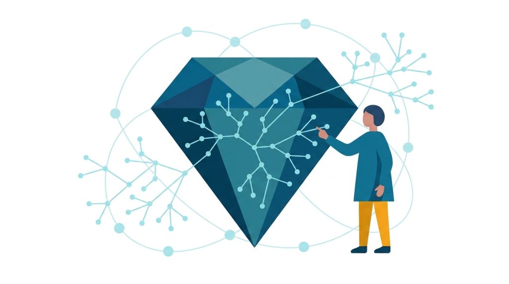
Fifty new customers just signed up. Your recommendation engine needs to place them into your graph’s embedding space today, not after tonight’s retraining job. This is the cold-start problem, and it’s the moment most embedding techniques fail.

Classic node embedding methods like Node2Vec or FastRP learn a separate vector for every node in the graph you trained on. So if you add a node, then there will be no vector for it. Your only option is to retrain on the whole graph again. GraphSAGE was built to remove that constraint, and Aura Graph Analytics provides a place to store the trained model so you can reuse it. Together, they turn “retrain the whole pipeline” into “call GraphSAGE on the new data.”

In this post, we’ll walk through GraphSAGE at a conceptual level, build a synthetic e-commerce graph to train on, and then use Aura Graph Analytics’ model catalog to generate embeddings for customers the model has never seen, without retraining anything.

If you would like a deep dive into how GraphSAGE works, check out the companion blog, “Understanding GraphSAGE” here.

What GraphSAGE actually does

Most node embedding algorithms need to retrain across the entire graph when new entities are added. So for every batch of new customers, you will need to retrain your embeddings. For many teams, this style of batch analytics works well, especially with efficient algorithms like FastRP.

GraphSAGE learns a function to generate embeddings during training, allowing it to apply that function to unseen nodes. For each node, it samples a fixed number of neighbors, pulls in their features, and combines them through a small neural network. Stack a few of these layers, and a node’s embedding ends up encoding not just its own features, but a summary of its neighborhood and its neighbors’ neighborhoods.

Because the output is a learned function of local structure and node features, rather than a memorized vector, you can hand that function a node it has never seen. As long as the node has features and at least one connection into the graph, it will produce a usable embedding. That’s what makes GraphSAGE inductive, and it’s why it’s worth reaching for transductive methods when your graph keeps growing.

A few parameters matter when you’re tuning it:

Aggregator: how a node combines its neighbors’ embeddings. Mean is fast and works well as a default; Pool captures richer neighborhood structure at a higher cost.
Sample sizes: how many neighbors get sampled per layer. Two layers with sample sizes like [25, 10] means each node looks at up to 25 direct neighbors and, through them, up to 10 of their neighbors.
Embedding dimension: the size of the output vector. Bigger captures more, but costs more to compute and store.
Epochs and tolerance: standard training controls for how long the model trains and when it decides it has converged.

None of this requires deep familiarity with neural networks to use well. You mostly need good node features and a sense of how many neighborhood-context hops matter for your problem.

The dataset: a small e-commerce graph with a cold-start twist

Everything else in this post runs on a single synthetic e-commerce graph, split into two waves so the cold-start problem actually occurs partway through rather than just being described.

Wave one, the training graph:

customers.csv: 500 customers with age, accountTenureDays, avgSessionMinutes, marketingOptIn
products.csv: 120 products with category, price, popularityScore
purchases.csv: ~3,700 (Customer)-[:PURCHASED]->(Product) edges with amount and rating
referrals.csv: 300 (Customer)-[:REFERRED]->(Customer) edges, skewed toward long-tenure customers

Wave two, the cold-start batch (arrives after training):

new_customers.csv: 50 brand-new customers, one to two days old
new_purchases.csv: their first purchases, connecting them into the existing product catalog

Purchase volume is weighted so tenured customers and popular products show up more often, and pricing follows a lognormal distribution, so the graph has the lumpy, skewed shape real commerce data has instead of a uniform toy distribution.

You can find a notebook with all the code, along with the generator script for our sample dataset (generate_dataset.py), and all six CSVs in this repository.

Before loading the data, you need an AuraDB instance configured to use Aura Graph Analytics. You should add the credentials to a .env file, so you can follow along.

Spinning up Aura Graph Analytics

You will be running almost all of your code in a python notebook, and will use an Aura Graph Analytics session to communicate with your AuraDB instance. Start by spinning one up!

import os
from dotenv import load_dotenv
from graphdatascience.session import GdsSessions, AuraAPICredentials, DbmsConnectionInfo, AlgorithmCategory
from datetime import timedelta

load_dotenv()

# This credential is the Organization ID
PROJECT_ID = os.environ["PROJECT_ID"]

# These credentials were generated after the creation of the Aura Instance
NEO4J_URI = os.environ["NEO4J_URI"]
NEO4J_USERNAME = os.environ.get("NEO4J_USERNAME", "neo4j")
NEO4J_PASSWORD = os.environ["NEO4J_PASSWORD"]

# These credentials were generated after the creation of the API Endpoint
CLIENT_SECRET = os.environ["CLIENT_SECRET"]
CLIENT_ID = os.environ["CLIENT_ID"]

sessions = GdsSessions(api_credentials=AuraAPICredentials(CLIENT_ID, CLIENT_SECRET, PROJECT_ID))

memory = sessions.estimate(
    node_count=1000, relationship_count=5000,
    algorithm_categories=[AlgorithmCategory.CENTRALITY, AlgorithmCategory.NODE_EMBEDDING],
)

db_connection_info = DbmsConnectionInfo(NEO4J_URI, NEO4J_USERNAME, NEO4J_PASSWORD)

session_name = "vscode"

# Initialize a GDS session scoped for 2 hours, sized to estimated graph
gds = sessions.get_or_create(
    session_name,
    memory=memory,
    db_connection=db_connection_info,
    ttl=timedelta(hours=1),
)

print("GDS session initialized.")
Code language: PHP (php)

Note: Credentials live in a .env file (loaded here with python-dotenv)

Next, load in your sample data. Load in customers.csv:

LOAD CSV WITH HEADERS FROM 'https://github.com/neo4j-product-examples/aura-graph-analytics/tree/main/graphsage/customers.csv' AS row
MERGE (c:Customer {customerId: row.customerId})
SET c.age = toInteger(row.age),
    c.accountTenureDays = toInteger(row.accountTenureDays),
    c.avgSessionMinutes = toFloat(row.avgSessionMinutes),
    c.marketingOptIn = toInteger(row.marketingOptIn);
Code language: PHP (php)

Load in products.csv:

LOAD CSV WITH HEADERS FROM 'https://github.com/neo4j-product-examples/aura-graph-analytics/tree/main/graphsage/products.csv' AS row
MERGE (p:Product {productId: row.productId})
SET p.name = row.name,
    p.category = row.category,
    p.price = toFloat(row.price),
    p.popularityScore = toFloat(row.popularityScore);
Code language: PHP (php)

Load in purchases.csv:

LOAD CSV WITH HEADERS FROM 'https://github.com/neo4j-product-examples/aura-graph-analytics/tree/main/graphsage/purchases.csv' AS row
MATCH (c:Customer {customerId: row.customerId}), (p:Product {productId: row.productId})
MERGE (c)-[r:PURCHASED]->(p)
SET r.amount = toFloat(row.amount), r.rating = toInteger(row.rating);
Code language: PHP (php)

Load in referrals.csv:

LOAD CSV WITH HEADERS FROM 'https://github.com/neo4j-product-examples/aura-graph-analytics/tree/main/graphsage/referrals.csv' AS row
MATCH (r:Customer {customerId: row.referrerId}), (e:Customer {customerId: row.refereeId})
MERGE (r)-[:REFERRED]->(e);Code language: PHP (php)

Every load here is MERGE on the identifying key, with the rest of each row’s fields applied via SET afterward, so rerunning these cells against a database that already has the data updates it in place instead of duplicating it.

Project the training graph into the session. Because customers and products carry different properties, use GraphSAGE’s multi-label mode, which projects each label’s features into a shared feature space via projected_feature_dimension:

gds.graph.drop("customer-graph", fail_if_missing=False)

G, result = gds.graph.project.cypher(
    graph_name="customer-graph",
    query="""
    CALL () {
        MATCH (c:Customer)-[r:PURCHASED]->(p:Product)
        RETURN c AS source, r AS rel, p AS target,
               c { .age, .accountTenureDays, .avgSessionMinutes, .marketingOptIn } AS sourceNodeProperties,
               p { .price, .popularityScore } AS targetNodeProperties
        UNION
        MATCH (c1:Customer)-[r:REFERRED]->(c2:Customer)
        RETURN c1 AS source, r AS rel, c2 AS target,
               c1 { .age, .accountTenureDays, .avgSessionMinutes, .marketingOptIn } AS sourceNodeProperties,
               c2 { .age, .accountTenureDays, .avgSessionMinutes, .marketingOptIn } AS targetNodeProperties
    }
    RETURN gds.graph.project.remote(source, target, {
      sourceNodeLabels: labels(source),
      targetNodeLabels: labels(target),
      sourceNodeProperties: sourceNodeProperties,
      targetNodeProperties: targetNodeProperties,
      relationshipType: type(rel),
      relationshipProperties: properties(rel)
    })
    """,
)
Code language: PHP (php)

Training GraphSAGE and landing it in the model catalog

This is where the model actually gets built, and where everything else in this post becomes possible: train once, and the model lands in the model catalog under the name you give it, ready to be called again later on customers it’s never met, no retraining required. Take a look at the parameters:

feature_properties lists what the model reads for each node: four properties for customers (age, how long they’ve been a customer, average time spent per visit, and whether they opted into marketing), and two for products (price and how popular it is).
projected_feature_dimension= 6 gives customers and products a shared way to be compared, even though they don’t have the same properties. GraphSAGE turns both into a 6-number description, one number per property in the list above, so no property gets left out.
aggregator= "Mean" controls how a node combines what it learns from its neighbors. Mean is the simpler, faster of the two options GraphSAGE offers, and it’s enough for a graph this size. The other option, Pool, picks up more detail but costs more to train.
activation_function= "Sigmoid" is left at Neo4j’s default setting here rather than changed.
sample_sizes: [25, 10] controls how many neighbors the model looks at, two steps out. Most customers here bought around 7 products, so checking up to 25 direct connections covers nearly everyone. The second step is capped lower, at 10, because that number grows fast: each of those 25 products brings its own list of customers along with it.
embedding_dimension= 64 sets the size of the description GraphSAGE builds for each node. 64 numbers is enough to hold the 6 input properties plus some neighborhood context, without being larger than this dataset needs.
random_seed=42 makes the training repeatable. Run it again with the same seed and you get the same result.

model, train_result = gds.graph_sage.train(
    G,
    model_name="customers",
    feature_properties=["age", "accountTenureDays", "avgSessionMinutes", "marketingOptIn", "price", "popularityScore"],
    projected_feature_dimension=6,
    aggregator="Mean",
    activation_function="Sigmoid",
    sample_sizes=[25, 10],
    embedding_dimension=64,
    random_seed=42,
)
Code language: JavaScript (javascript)

The catalog is what makes a trained model reusable: you can inspect what’s registered, confirm how it was trained, and check it’s ready to use. Here’s what’s in the registry:

gds.model.list()Code language: CSS (css)

Fetch the trained model back from the catalog:

model = gds.model.get("customers")Code language: JavaScript (javascript)

Write the training embeddings back to your AuraDB. You’ll use them later for KNN:

gds.graph_sage.mutate(G, model_name="customers", mutate_property="embedding")
gds.graph.node_properties.write(G, ["embedding"])Code language: JavaScript (javascript)

New customers, new embeddings, same model

Here is the cold-start problem in action: a new batch of customers just signed up. Previously, you’d need to retrain on the entire graph to generate embeddings for them. With GraphSAGE, you apply the weights and biases from the earlier training run directly to new customers.

First, load in the new customers:

gds.run_cypher("""
LOAD CSV WITH HEADERS FROM 'https://github.com/neo4j-product-examples/aura-graph-analytics/tree/main/graphsage/new_customers.csv' AS row
CREATE (:Customer {
  customerId: row.customerId,
  age: toInteger(row.age),
  accountTenureDays: toInteger(row.accountTenureDays),
  avgSessionMinutes: toFloat(row.avgSessionMinutes),
  marketingOptIn: toInteger(row.marketingOptIn)
});
               """)Code language: PHP (php)

Load in the new purchases:

gds.run_cypher("""
LOAD CSV WITH HEADERS FROM 'https://github.com/neo4j-product-examples/aura-graph-analytics/tree/main/graphsage/new_purchases.csv' AS row
MATCH (c:Customer {customerId: row.customerId}), (p:Product {productId: row.productId})
CREATE (c)-[:PURCHASED {amount: toFloat(row.amount), rating: toInteger(row.rating)}]->(p);                     
               """)Code language: PHP (php)

Project the new customers into a graph, so you can run the trained GraphSAGE model against them:

G_new, _ = gds.graph.project.cypher(
    graph_name="new-customer-graph",
    query="""
    MATCH (c:Customer)-[r:PURCHASED]->(p:Product)
    WHERE c.customerId STARTS WITH 'N'
    RETURN gds.graph.project.remote(c, p, {
      sourceNodeLabels: labels(c),
      targetNodeLabels: labels(p),
      sourceNodeProperties: c { .age, .accountTenureDays, .avgSessionMinutes, .marketingOptIn },
      targetNodeProperties: p { .price, .popularityScore },
      relationshipType: type(r),
      relationshipProperties: properties(r)
    })
    """,
)Code language: PHP (php)

Write the new embeddings back to the graph:

gds.graph_sage.mutate(G_new, model_name="customers", mutate_property="embedding")
gds.graph.node_properties.write(G_new, ["embedding"])Code language: JavaScript (javascript)

After this step, every Customer and Product node in AuraDB has an embedding property, old and new alike.

Calculating similarity scores

Embeddings are useful for similarity: nodes with similar embeddings share similar features and neighborhood structure. Here, measure that using K-nearest neighbors (KNN).

First, add labels to distinguish between new and old customers, then create a graph projection:

gds.run_cypher("MATCH (c:Customer) WHERE c.customerId STARTS WITH 'C' SET c:OldCustomer")
gds.run_cypher("MATCH (c:Customer) WHERE c.customerId STARTS WITH 'N' SET c:NewCustomer")

gds.graph.drop("embedded-graph", fail_if_missing=False)

G_embedded, _ = gds.graph.project.cypher(
    graph_name="embedded-graph",
    query="""
    MATCH (c:Customer)-[r:PURCHASED]->(p:Product)
    RETURN gds.graph.project.remote(c, p, {
      sourceNodeLabels: labels(c),
      targetNodeLabels: labels(p),
      sourceNodeProperties: c { .embedding },
      targetNodeProperties: p { .embedding },
      relationshipType: type(r),
      relationshipProperties: properties(r)
    })
    """,
)Code language: PHP (php)

Run K-nearest neighbors, then write the results back to the graph:

gds.knn.filtered.mutate(
    G_embedded,
    mutate_relationship_type="SIMILAR_TO",
    mutate_property="score",
    node_properties=["embedding"],
    source_node_filter="NewCustomer",
    target_node_filter="OldCustomer",
    top_k=1,
)

gds.graph.relationships.write(G_embedded, "SIMILAR_TO", ["score"])
Code language: JavaScript (javascript)

Finally, pull back the results with a Cypher query: which new customers most resemble existing ones.

gds.run_cypher(
    """
    MATCH (new:NewCustomer)-[r:SIMILAR_TO]->(old:OldCustomer)
    RETURN new.customerId AS newCustomer,
           old.customerId AS existingCustomer,
           r.score AS similarity
    ORDER BY similarity DESC
    """
)Code language: CSS (css)

A pair is similar because of their embeddings, which reflect features and neighborhood structure generally, not exclusively shared purchases, so it’s expected that most pairs won’t share a purchased product at all.

Wrap-up

You trained one GraphSAGE model and used it twice: once on the customers it was trained on, and once on fifty customers it had never seen. Same model, no retraining, both times producing embeddings ready for the similarity search above.

This is the pattern GraphSAGE is built for. Whenever your graph keeps growing (new customers, new transactions, new accounts), you don’t retrain from scratch every time something new shows up. You train periodically, then predict on demand.

Everything you need to run this yourself is included: the dataset generator, the CSVs, and the companion notebook. Spin up your own Aura Graph Analytics session from the Aura Console, swap in your AuraDB credentials, and watch the same cold-start scenario play out on your own data. If you get stuck, the GDS Python Client tutorials cover session setup in more depth.