From first graph algorithm experiment to production with Aura Graph Analytics

Many data teams have the same conversation about graph analytics: “That’s the fraud detection thing, right?” Then they go back to their pipelines, assuming that graph analytics isn’t relevant to their use cases or the data they’re working with.

It’s a reasonable shortcut, but a limiting one. Use cases like fraud detection, entity resolution, and customer 360 dominate the conversation because they’re proven, high-stakes, and relevant across industries, which is exactly why they overshadow a lot of other areas where graph algorithms would give you genuinely useful signals.

Most datasets have a connectivity aspect that tabular approaches fail to surface. These aspects don’t always map to a textbook graph analytics use case, and that’s fine. Today, you can get a concrete answer on where graph analytics adds value to your data in minutes, without needing deep algorithm expertise — and that’s exactly where this article starts. From there, we’ll cover how to run your first experiments, get your data in and out efficiently, and eventually turn the whole thing into a production pipeline.

The tool you’ll be using throughout this article is Aura Graph Analytics (AGA), Neo4j’s on-demand compute environment for running graph algorithms at scale. It’s built on top of the Graph Data Science (GDS) library; you can think of GDS as the algorithm engine, and AGA as the managed cloud infrastructure that runs it with minimal setup. In AGA, each session is a standalone compute unit: you create it, load data into it via a projection, run algorithms, write results back to your source, and then terminate it.

Finding the right algorithm for your data

Before writing any code, you need to start with the harder (and more important) questions: which category of graph problem do you actually have, and which algorithms are the most well-suited for your use case(s)?

Historically, these were questions that required you to do the extra work of connecting the dots. Today, however, your task is much simpler. Using either Aura’s built-in AI chat assistant (available in the Aura console) or any publicly available LLM like Claude or Gemini, you can describe your data and what you’re solving for and let the LLM navigate the world of graph algorithms and their use cases for you.

For best results, give it your node labels, relationship types, and what you’re trying to learn from the data. Something like: “I have Customer, Order, and Product nodes; Customers place Orders that contain Products. What Graph Data Science algorithms would add the most useful new properties or relationships here?” You’ll often get suggestions you wouldn’t have arrived at on your own.

Beyond the basic prompt, there are a few ways to get a lot more out of this step:

• If you’re using an LLM that supports MCP, connect it directly to your Neo4j instance. Instead of typing out your schema by hand, the LLM can inspect it directly and work from what’s actually there.
• If your data isn’t in graph format at all, or you’ve never thought about it as a graph, that’s fine. Describe it the way you naturally would (tables, columns, foreign keys, and so on), and the LLM can help translate that into a graph model and identify relevant graph algorithms for your use cases. When it’s time to run the algorithms, you can ingest data into Aura Graph Analytics from any source using pandas or Apache Spark DataFrames, with no migration required.
• For ready-to-use end-to-end scripts, connect the publicly available agent skills for Graph Data Science and Aura Graph Analytics to your LLM, so it can generate working code based on your actual data.

Once you have a shortlist, you can start experimenting with algorithms both visually and in code.

Your first experiment: three ways in

There are three ways to run your first experiment in AGA. The right one depends on where your data lives, how you prefer to work, and what you’re trying to validate.

Visual exploration with Bloom

If your data is already in AuraDB and you want the fastest possible path to seeing algorithm output, start in Bloom, Aura’s graph exploration tool. Via the intuitive Bloom UI, you can define the data you want to use, pick your algorithm, configure it visually, and run it. You can then easily style results to appear directly in the graph visualization (for example, using communities to color nodes or PageRank scores to scale node sizes).

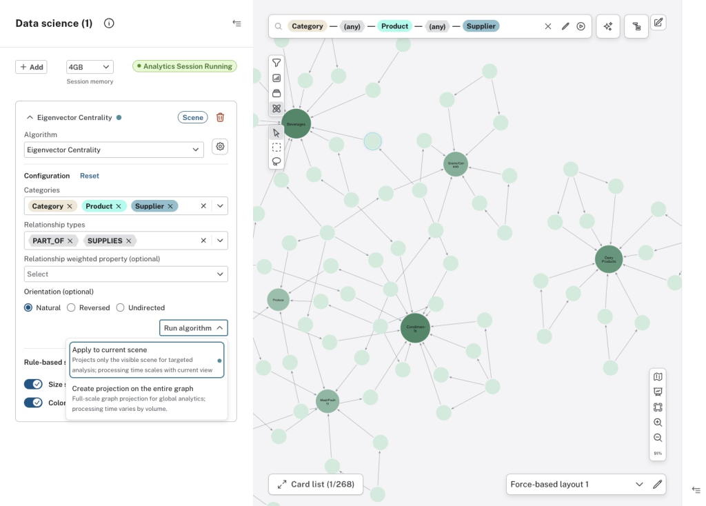
This visual path is the best and most accessible tool for validating whether an algorithm is producing meaningful structure on your data. It’s particularly useful for categories like community detection and centrality measures, where the output is inherently visual, and you want to sense-check it before investing in a pipeline.

By default, running an algorithm in Bloom only affects the visualization and nothing gets written to your data source. If you want to persist the results, you only need to flip a setting to run the algorithm on the entire graph instead, which also writes the result back as a real property on every affected element, not just the ones visible in the visualization.

Although Bloom doesn’t support automation or scheduling (yet), AGA offers other tools built for programmatic use cases. Its Cypher and Python interfaces, which we cover next, are where that happens.

For additional details on running AGA via Bloom, refer to the dedicated documentation page.

Cypher in the Query tool

For more precise control over algorithm configuration, or if you’re already comfortable writing Cypher, the Query tool in the Aura console is the next option. With it, you interact with Aura Graph Analytics directly via its Cypher procedures:

-- Project a graph into an AGA session
CALL gds.graph.project(
'customer-graph', 
'Customer',
'INTERACTED_WITH',
{
     memory: '2GB'
})

-- Run PageRank in stream mode to inspect scores
CALL gds.pageRank.stream('customer-graph')
YIELD nodeId, score
RETURN gds.util.asNode(nodeId).customerId AS id, score
ORDER BY score DESC
LIMIT 20Code language: PHP (php)

The advantage with this programmatic approach is that everything you test via Cypher translates directly to a production pipeline: AGA’s Cypher API is the same API whether you’re experimenting interactively or running scheduled jobs.

Python notebooks

For anything more complex (iterative experimentation, ML pipelines, data coming from non-Neo4j sources, etc.) or if you’re just more comfortable with Python than Cypher, then the GDS Python client is the interface best suited for the job. (Quick version note: all the Python code in this article uses GDS Python client 2.0 syntax.)

Start by installing the library in your working environment (using pip or a similar tool), then create an AGA session from the client. In the example below, we’re creating a session attached to an AuraDB database:

import os
from dotenv import load_dotenv 
from graphdatascience.session import (
    GdsSessions, AuraAPICredentials, DbmsConnectionInfo, SessionMemory
)

# Create Aura API credentials in your Aura console (under API credentials) first,
# then save them to a local .env file (the filenames below are just examples)
load_dotenv("api_credentials.env")  # point at the file containing Aura API credentials
load_dotenv("db_credentials.env")  # point at the file containing database credentials

# Entry point for creating and managing GDS sessions
sessions = GdsSessions(api_credentials=AuraAPICredentials(
    client_id=os.environ["CLIENT_ID"],
    client_secret=os.environ["CLIENT_SECRET"],
    project_id="my-project"
))

# Creating an AGA session
gds = sessions.get_or_create(
    session_name="my-experiment",
    memory=SessionMemory.m_8GB,
    db_connection=DbmsConnectionInfo(
        aura_instance_id=os.environ["AURA_INSTANCE_ID"],
        username=os.environ["NEO4J_USERNAME"],
        password=os.environ["NEO4J_PASSWORD"]
    )
)Code language: PHP (php)

The get_or_create() call is idempotent: if a session with that name already exists, it reconnects to it rather than creating a new one. This becomes particularly useful when you’re reconnecting between pipeline steps, which we’ll cover later.

The Python client API mirrors the Cypher API closely. For example, here’s what running Louvain community detection and FastRP embeddings looks like:

G, results = gds.graph.project.native(
    "customer-graph",
    node_label_filter=["Customer"],
    relationship_type_filter=["INTERACTED_WITH"],
)
gds.louvain.mutate(G, mutate_property="community")
gds.fast_rp.mutate(
    G,
    feature_properties=["community"],
    embedding_dimension=128,
    mutate_property="embedding"
)Code language: JavaScript (javascript)

For in-notebook visualization, the neo4j-viz package integrates directly with GDS projected graphs via its from_gds() helper function:

from neo4j_viz.gds import from_gds

VG = from_gds(gds, G, db_node_properties=["name"])
for node in VG.nodes:
    node.caption = node.properties.get("name")

VG.render_widget(initial_zoom=1.2)Code language: JavaScript (javascript)

This renders an interactive graph in the notebook cell, so you can visually check whether the algorithm output makes sense on your data before building anything further. See the neo4j-viz documentation for more on customizing node size, color, and captions.

Getting data in and out efficiently

Once you’ve confirmed that one or more algorithms make sense for your data, the next step is to make the projection and write-back as efficient as possible. These steps represent both the process of moving data between your source system and the AGA session and the transformation of the data to and from a compressed sparse format optimized for graph traversal. For large graphs, projection often accounts for the majority of the total runtime, so this step is worth some attention.

Remote projection from a Neo4j source

For AGA sessions which run on top of Neo4j sources (both Aura and self-managed Neo4j), you load data via a remote projection. The query runs on your Neo4j database but streams data into the AGA session:

G, result = gds.graph.project.cypher(
    "customer-graph",
    """
    MATCH (c:Customer)-[r:INTERACTED_WITH]->(c2:Customer)
    RETURN gds.graph.project.remote(c, c2, {
        sourceNodeLabels: labels(c),
        targetNodeLabels: labels(c2),
        relationshipType: type(r),
        sourceNodeProperties: c {.tenure, .segment},
        targetNodeProperties: c2 {.tenure, .segment}
    })
    """,
)Code language: PHP (php)

The query above is a Cypher projection: thanks to MATCH/RETURN logic, you benefit from full flexibility over what gets projected. You can filter to a subgraph, compute derived properties on the fly, or handle heterogeneous structures with UNION clauses. If your graph is straightforward and you just want to project everything for a given label and relationship type, the query simplifies considerably.

For additional performance, you can prefix the query with CYPHER runtime=parallel to use the parallel Cypher runtime on multi-core AuraDB instances. You can also tune batch_size and concurrency on the gds.graph.project.cypher() call itself to control how data is batched and transferred between the database and the session.

However, when working with large graphs and fairly simple projections (i.e. without any advanced filtering logic), you should instead opt for Native projections. These projections read data directly from the disk and don’t have to execute any query logic, thereby drastically improving performance, especially at scale.

For Python, the full remote projection syntax is documented in the AGA Python client reference.

Loading from Pandas or Apache Spark (standalone sessions)

If your data source is Databricks, Apache Iceberg, a data warehouse, or anything non-Neo4j, use a standalone session and gds.graph.construct() with Pandas or Apache Spark DataFrames. For Apache Spark, a detailed example is available via the Python client docs. As for Pandas, the below example shows the end-to-end process:

import pandas as pd
import os
from dotenv import load_dotenv
from graphdatascience.session import (
    CloudLocation, SessionMemory, GdsSessions, AuraAPICredentials
)

load_dotenv("api_credentials.env")

sessions = GdsSessions(api_credentials=AuraAPICredentials(
    client_id=os.environ["CLIENT_ID"],
    client_secret=os.environ["CLIENT_SECRET"],
    project_id="my-project"
))

gds = sessions.get_or_create(
    session_name="standalone-session",
    memory=SessionMemory.m_16GB,
    cloud_location=CloudLocation(provider="gcp", region="us-east1")
)

# One row per node: nodeId and labels are required, the rest are node properties
nodes = pd.DataFrame({
    "nodeId": customer_df["id"].tolist(),
    "labels": ["Customer"] * len(customer_df),
    "tenure": customer_df["tenure"].tolist(),
    "segment": customer_df["segment"].tolist()
})

# One row per relationship: source/target node IDs and type are required, plus any properties
relationships = pd.DataFrame({
    "sourceNodeId": edges_df["source_id"].tolist(),
    "targetNodeId": edges_df["target_id"].tolist(),
    "relationshipType": edges_df["type"].tolist(),
    "weight": edges_df["weight"].tolist()
})

G = gds.graph.construct("customer-graph", [nodes], [relationships])Code language: PHP (php)

This pattern fits neatly into broader data pipelines: read from table A in Snowflake, run graph analytics, write enriched results to table B, with no Neo4j database required as a data store.

Writing results back

For sessions connected to Neo4j data sources, writing computed properties back to the database is a single call:

# Write specific properties computed during the session
gds.graph.node_properties.write(G, ["community", "embedding"])

# Or use write mode on the algorithm directly
gds.louvain.write(G, write_property="community")Code language: PHP (php)

For standalone sessions, stream results back to a DataFrame and write them wherever you need:

results_df = gds.graph.node_properties.stream(
    G, ["community", "embedding"],
    separate_property_columns=True
)
# write results_df to Snowflake, Apache Iceberg, a feature store, etc.Code language: PHP (php)

Right-sizing your session

AGA allows you to choose the size of every session, ensuring maximum flexibility and that the session you’re paying for truly matches your workload. However, figuring out which size to specify based on the algorithms you plan to run and your data volume requires knowledge about every algorithm’s memory requirements. Luckily, AGA provides the estimate() method, which takes your expected data size and the algorithm(s) you plan to use, and returns a recommended memory tier:

from graphdatascience.session import AlgorithmCategory

memory = sessions.estimate(
    node_count=5000,
    relationship_count=25000,
    algorithms={
      "wcc": {}, 
      "fast_rp": {"embedding_dimension": 1024}
    },
    node_property_count=5,
    relationship_property_count=2
)

print(f"Recommended: {memory}")  # e.g., SessionMemory.m_32GBCode language: PHP (php)

The estimation covers both the projection and the algorithm execution, ensuring the risk of an out-of-memory scenario is minimal.

The full estimation documentation for AGA is available here.

Running it in production

You’ve validated the algorithm, tuned the projection, and confirmed an ideal session size. The last piece is to turn this into a pipeline that runs automatically on fresh data.

Scheduled execution

The GDS Python client is just Python, so it runs anywhere Python runs. The simplest production pattern is a script in a scheduled environment: a managed notebook service like Vertex AI Workbench, a cron job, or directly as an Apache Airflow task using PythonOperator. The below example shows a basic Apache Airflow DAG containing an AGA step:

from airflow import DAG
from airflow.operators.python import PythonOperator
from datetime import datetime

def run_graph_analytics():
    import os
    from graphdatascience.session import (
        GdsSessions, AuraAPICredentials, DbmsConnectionInfo, SessionMemory
    )

    sessions = GdsSessions(api_credentials=AuraAPICredentials(
        os.environ["CLIENT_ID"], os.environ["CLIENT_SECRET"], "my-production-project"
    ))
    gds = sessions.get_or_create(
        session_name="daily-analytics",
        memory=SessionMemory.m_16GB,
        db_connection=DbmsConnectionInfo(
            aura_instance_id=os.environ["AURA_INSTANCE_ID"],
            username=os.environ["NEO4J_USERNAME"],
            password=os.environ["NEO4J_PASSWORD"]
        )
    )

    G, _ = gds.graph.project.cypher("customer-graph", PROJECTION_QUERY)
    gds.louvain.write(G, write_property="community")
    gds.fast_rp.write(G, write_property="embedding", embedding_dimension=128)
    gds.delete()

with DAG(
    "graph_analytics",
    schedule_interval="0 2 * * *",
    start_date=datetime(2026, 1, 1),
    catchup=False
) as dag:
    PythonOperator(task_id="run_analytics", python_callable=run_graph_analytics)Code language: JavaScript (javascript)

Thanks to AGA’s default Time-To-Live (ttl) setting of one hour, even if the script fails mid-run and never calls gds.delete(), the session expires automatically after the configured period and stops incurring costs. If you want to minimize risks even further, you can set a more restrictive TTL, like 10 minutes for example.

Async execution for longer workflows

For larger graphs, projection can take several minutes to hours. Running the entire workflow as a single synchronous task, with this constraint, is fragile — given that a transient failure partway through means restarting from the beginning.

The better approach is to split the pipeline into distinct steps with explicit handoffs between the different operations: Step 1 triggers the projection, step 2 waits for it to complete, step 3 runs the algorithms once the graph is ready, and finally step 4 handles write-back and cleanup.

In AGA, this is possible thanks to the asynchronous execution endpoints. An Apache Airflow implementation of this approach would, for example, use PythonSensor for the wait step, and because the get_or_create() function reconnects to an existing session by name, each task can reconnect independently without sharing state between Apache Airflow operators.

Session resizing

A session size that works today won’t necessarily work in six months. As your data grows, jobs run longer, and eventually an undersized session hits an OOM error in production (usually at the worst possible time).

The right habit is to regularly re-evaluate the session size so you know when an upsize is needed, before it becomes urgent. Good signals to watch for include job duration trending up over time and data volume crossing meaningful thresholds (a 2x growth in node or relationship count is a reasonable trigger to re-run an estimate).

The sessions.estimate() helper function makes this straightforward. You can run it as a recurring process that matches your data growth pace (via a weekly Apache Airflow DAG or a scheduled notebook) or using a simple Cypher call in the Query tool if you want something quick and manual.

When you call the function, the output tells you whether your current session size still makes sense. If the recommendation has jumped a tier, that’s your cue to upsize before the next production job to ensure things continue to run smoothly.

Putting it together

The path from “this might work for my data” to “this runs every night in production” is shorter than it looks. The most important part happens early on, and is simpler (and more efficient) than ever thanks to LLMs: finding the right algorithm and confirming it produces a useful signal on your actual data. Once that’s done, the rest is mostly connecting the pieces you already have.

Start in Bloom or the Query tool to validate the idea visually, move to the Python client for precise configuration and notebook-based iteration, use sessions.estimate() to size the session correctly, and deploy via whatever scheduler your team already runs. The AGA Python tutorials have ready-to-run notebooks for each session type (attached, self-managed, and standalone) if you want working code in your hands quickly.

Aura Graph Analytics is available on Aura’s free tier, so you can create an account for free and follow along with every step in this article without any setup cost. If you want a structured walkthrough of the console and Python workflows covered above, GraphAcademy’s new AGA fundamentals course covers the same ground in about an hour. (It assumes you’ve completed GDS fundamentals first, so start there if GDS is completely new to you.) To take things even further, the hands-on AGA workshop picks up right where this article leaves off.

---

From first graph algorithm experiment to production with Aura Graph Analytics was originally published in Neo4j Developer Blog on Medium, where people are continuing the conversation by highlighting and responding to this story.