Auditing AWS infrastructure with Neo4j: questions inventory cannot answer

Somebody asks whether GuardDuty covers every account. The question is about holes in the coverage, not about whether the service is switched on. From a flat resource inventory that is a genuinely annoying question. You export accounts, export detectors, line them up in a spreadsheet, and the answer is stale the moment anyone runs terraform apply.

It is annoying because it is not an inventory question. It asks about a missing relationship between two things you already have, and a list is the wrong shape for that. A relationship here is a conceptual claim as much as a stored fact. It records what the estate is meant to do, where that intent came from, and how it is enforced. A detector’s scope asserts coverage, and security group rules and routes assert reachability, both of them typically expressed as rules or infrastructure as code. Modelling an edge means modelling that intent next to the observation.

Most questions worth asking about an estate are like this. Which internet-facing thing reaches the database. Which accounts can genuinely reach each other, whatever the network diagram claims.

The audit boundary is the set of accounts a compliance scope such as SOC 2 covers, which is usually narrower than the set of accounts the company owns. An account inside that boundary is in scope, and one outside it is not. The estate here includes an acquired account that has never been brought inside the boundary, and it is where the reachability and segmentation queries find their results.

This article builds the graph that answers those questions, then hands it to an agent. An agent pointed at it re-derives the same conclusions nightly, so the last section gives it a memory.

Collecting the inventory

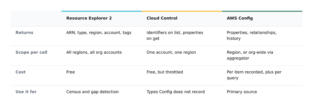
The API you start from matters. Resource Explorer 2 returns an ARN, a type, a region, an account, and tags. That is a node list with no properties, so it gives you no edges. Every edge below comes from configuration data, including reachability from security group rules and routes, role attachment from task definitions, and encryption from bucket settings.

AWS Config supplies exactly that, so make it your primary source. Each configuration item carries configuration and a relationships block, and select-aggregate-resource-config runs org-wide through an aggregator.

aws configservice select-aggregate-resource-config \
  --configuration-aggregator-name org-aggregator \
  --expression "SELECT resourceId, resourceType, configuration, relationships \
                WHERE resourceType = 'AWS::ECS::Service'" \
  --limit 100

Resource Explorer is the cheap independent census you check Config against. It is free, spans accounts and regions in one call, and answers “what exists that Config is not recording?” Setup needs an index per account, an aggregator index, and Organizations trusted access.

Cloud Control is the one people reach for first and the one to reach for last. Its uniform CloudFormation-registry schema means one parser handles every type, but list-resources returns identifiers rather than properties, so each resource needs a further get-resource call against the most throttled of the three APIs. Reserve it for the types Config does not record. Not all of the 2,082 public types in us-east-1 are enumerable, and AWS::ECS::TaskSet has no list handler at all:

aws cloudformation describe-type --type RESOURCE \
  --type-name AWS::ECS::TaskSet --query Schema --output text | jq '.handlers | keys'
# ["create","delete","read","update"]        <- no "list"

A flat resource graph cannot answer these questions

A Config dump maps very naturally onto one node type and one relationship type. That is the modelling mistake that makes everything downstream harder:

(:Resource {arn, type, ...})-[:RELATED_TO]->(:Resource)

It loads fast and it even looks like a graph, but it is nearly useless, because RELATED_TO between a subnet and an instance means something different from RELATED_TO between a policy and a bucket, so every query has to rebuild that difference from properties.

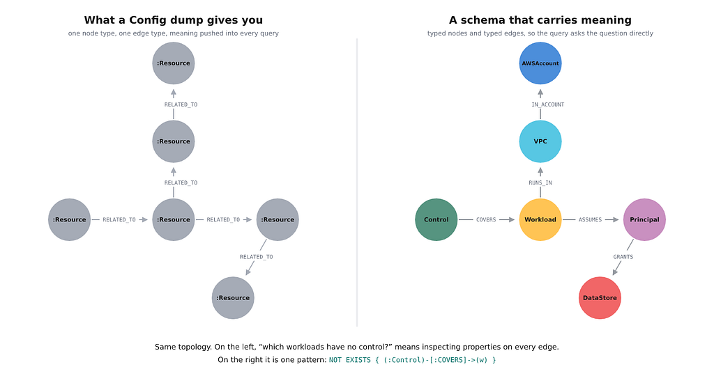
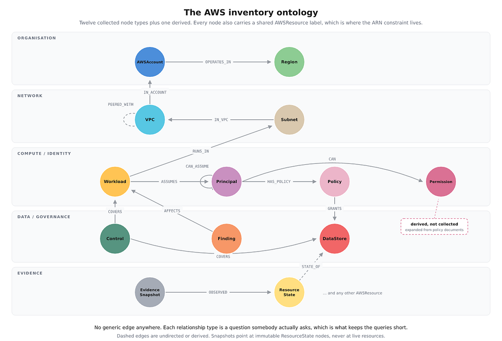
Typed nodes keep that meaning in the graph. Twelve collected node types, plus one derived, in the shape create-context-graph uses:

domain:
  id: aws-inventory
  name: AWS Inventory

entity_types:
  - label: AWSAccount
    pole_type: ORGANIZATION
    properties:
      - {name: accountId, type: string, required: true, unique: true}
      - {name: alias, type: string}
      - {name: complianceScopes, type: list}
  
  - label: Workload
    pole_type: OBJECT
    subtype: IT_ASSET
    properties:
      - {name: arn, type: string, required: true, unique: true}
      - {name: type, type: string,
         enum: [ec2_instance, ecs_service, lambda, eks_pod, alb, nlb, api_gateway]}
      - {name: internetFacing, type: boolean}

  - label: DataStore
    pole_type: OBJECT
    subtype: DATA_ASSET
    properties:
      - {name: arn, type: string, required: true, unique: true}
      - {name: dataClass, type: string,
         enum: [customer-pii, secret, operational, public, none]}
      - {name: encrypted, type: boolean}

# Derived from expanded policy statements, not collected from AWS.
  - label: Permission
    pole_type: OBJECT
    properties:
      - {name: action, type: string, required: true, unique: true}

The rest follow the same pattern, including Region, VPC, Subnet, Principal, Policy, Control, Finding, ResourceState, and EvidenceSnapshot. Each relationship carries a specific type. This listing is plain text because label alternation like (:Workload|:DataStore) is invalid in a node pattern:

(:AWSAccount)-[:OPERATES_IN]->(:Region)
(:VPC)-[:IN_ACCOUNT]->(:AWSAccount)
(:Subnet)-[:IN_VPC]->(:VPC)
(:Workload)-[:RUNS_IN]->(:Subnet)
(:Workload)-[:ASSUMES {via}]->(:Principal)
(:Principal)-[:CAN_ASSUME {mfaRequired, externalId, conditionCount}]->(:Principal)
(:Principal)-[:HAS_POLICY]->(:Policy)
(:Principal)-[:CAN {effect}]->(:Permission)
(:Policy)-[:GRANTS {effect, action, conditionCount}]->(:DataStore)
(:Workload)-[:REACHES {protocol, fromPort, toPort, cidr}]->(:Workload)
(:VPC)-[:PEERED_WITH {peeringId}]-(:VPC)
(:Control)-[:COVERS]->(:Workload)
(:Finding)-[:AFFECTS]->(:Workload)
(:EvidenceSnapshot)-[:OBSERVED]->(:ResourceState)
(:ResourceState)-[:STATE_OF]->(:AWSResource)

Some parts of that schema do specific work. complianceScopes holds a list, since one account can be in scope for SOC 2, an internal policy, and a customer contract at once, with different owners and review cycles, and each of those scopes has to stay addressable on its own.

An EvidenceSnapshot points at ResourceState nodes, each of them immutable once written. The nightly run mutates resources in place, so pinning an observation to a fixed state is what keeps last month’s snapshot describing last month.

Control -[:COVERS]-> makes absence queryable. The useful answer to a coverage question is which workloads have no GuardDuty edge, and a RELATED_TO model cannot produce that without teaching every query what monitoring looks like.

Loading

The shared AWSResource label carries the ARN constraint, so uniqueness is declared once for every type. Dynamic labels then let one statement handle the load.

CREATE CONSTRAINT aws_resource_arn IF NOT EXISTS
FOR (n:AWSResource) REQUIRE n.arn IS UNIQUE;

Nodes then load in batches, with one statement for every type. The label arrives as data in each row, so a single statement covers all twelve types:

UNWIND $batch AS row
MERGE (n:AWSResource {arn: row.arn})
SET n:$(row.label),
    n += row.properties
RETURN count(n) AS loaded;

SET n:$(row.label) takes the label as a value, so nothing is spliced into the query text. Dynamic labels scan and filter where a static label would use an index, which keeps this in a loader and off a hot read path.

Edges load the same way, as a plain batch. Both endpoints are matched by ARN, so the nodes have to be in place before this runs:

UNWIND $edges AS edge
MATCH (a:AWSResource {arn: edge.from})
MATCH (b:AWSResource {arn: edge.to})
MERGE (a)-[r:REACHES]->(b)
SET r += edge.properties;

An estate this size needs nothing more. At volumes where edge writes start contending, the same block goes inside CALL { … } IN CONCURRENT TRANSACTIONS with ON ERROR RETRY, because every edge write touches two nodes and parallel batches collide.

Queries the model unlocks

Everything below runs against a synthetic estate. Halyard is a B2B subscription billing platform, with a public gateway and subscription API in halyard-edge, billing and statement exports in halyard-billing, and an EU residency stack in halyard-eu. Nine months ago it acquired Pinemark Analytics, whose stack still runs in pinemark-legacy. That account has never been audited, and its VPC is peered into billing for an unfinished migration.

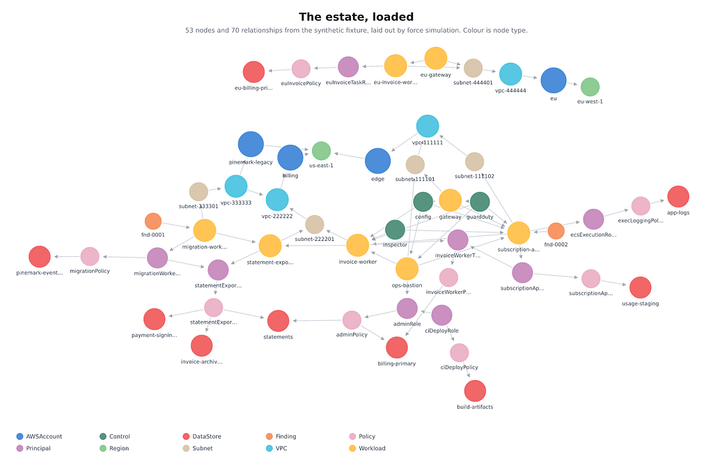
The EU stack sits on its own, with no edge joining it to the rest. The other three accounts form a single cluster, so they are less separate than the account boundary implies, and the segmentation check turns that into a finding.

Coverage gaps

The GuardDuty question from the opening, as a query. It asks for the absence of a relationship, which the COVERS edge makes directly queryable.

MATCH (a:AWSAccount) WHERE 'soc2' IN a.complianceScopes
MATCH (w:Workload)-[:RUNS_IN]->(:Subnet)-[:IN_VPC]->(:VPC)-[:IN_ACCOUNT]->(a)
WHERE NOT EXISTS { (:Control {id:'guardduty-us-east-1'})-[:COVERS]->(w) }
RETURN a.alias AS account, w.type AS type, w.arn AS uncovered
ORDER BY uncovered;

account,           type,          uncovered
"halyard-eu",      "ecs_service", "arn:aws:ecs:eu-west-1:444444444444:service/prod/eu-invoice-worker"
"halyard-eu",      "alb",         "arn:aws:elasticloadbalancing:eu-west-1:444444444444:loadbalancer/app/eu-gateway/123456"
"halyard-billing", "lambda",      "arn:aws:lambda:us-east-1:222222222222:function:statement-export"

Nothing is watching those three workloads. The lambda was added after coverage was last reviewed. Both EU workloads are missing because GuardDuty is regional and this detector lives in us-east-1, so it covers nothing in eu-west-1. An account-by-account view of whether GuardDuty is enabled does not show that gap, because the region has to be part of the check.

Bounded reachability

Which internet-facing things can reach customer data, and how directly. This walks REACHES edges for up to four hops.

MATCH p = ACYCLIC (src:Workload)-[:REACHES]->{1,4}(dst:Workload)
WHERE src.internetFacing = true
MATCH (dst)-[:ASSUMES]->(:Principal)-[:HAS_POLICY]->(:Policy)-[:GRANTS]->(ds:DataStore)
WHERE ds.dataClass = 'customer-pii'
RETURN last(split(src.arn,':')) AS entry, length(p) AS hops,
       last(split(dst.arn,':')) AS via, last(split(ds.arn,':')) AS reached
ORDER BY hops, entry LIMIT 6;

entry,                                 hops, via,                           reached
"instance/i-123456",                   1,    "service/prod/invoice-worker", "billing-primary"
"loadbalancer/app/eu-gateway/123456",  1,    "service/prod/eu-invoice-worker","eu-billing-primary"
"service/migration/migration-worker",  1,    "statement-export",            "halyard-statements"
"instance/i-123456",                   2,    "service/prod/invoice-worker", "billing-primary"
"instance/i-123456",                   2,    "statement-export",            "halyard-statements"
"loadbalancer/app/gateway/123456",     2,    "service/prod/invoice-worker", "billing-primary"

The first two rows are expected. Both entry points are Halyard’s own gateways reaching billing data inside the audit boundary. The third row is different, because its entry point sits in pinemark-legacy, the acquired account outside the boundary, and it is one hop from customer statements.

ACYCLIC stops a path revisiting a node. Reachability graphs are full of mutual security group rules, where two workloads each allow the other, and without that keyword those pairs generate looping paths that pad the result with nothing new.

One caveat applies to every result above. These REACHES edges come from security group rules, routes, and listener configuration, so they describe network exposure. Authorization is a separate layer, and proving that a path is exploitable means evaluating IAM policy with Deny precedence and condition blocks, which this schema does not attempt and which is a substantial piece of work on its own. Treat each row as a candidate to check. Whether the accounts are segmented at all is a separate question, and an algorithm answers it better than a traversal.

Graph algorithm: segmentation

The reachability query answers questions about specific paths. Segmentation is a question about the whole estate. It asks which workloads sit in one connected group, and whether any of those groups straddles the audit boundary. Clustering answers that in a single pass over the whole graph. The projections here run on Aura Graph Analytics, the serverless form of GDS, which is why they carry a memory key.

Weakly Connected Components is the cheap way to get those groups. It treats every edge as undirected and puts two workloads in the same component when any path joins them. Ignoring direction errs toward overstating connection, so the result never reports two things as separated when they are not. Project the reachability edges, then look for a component that mixes things which should not be able to talk.

MATCH (a:Workload)-[:REACHES]->(b:Workload)
RETURN gds.graph.project('netseg', a, b, {},
  {undirectedRelationshipTypes: ['*'], memory: '2GB'}) AS g;

CALL gds.wcc.stream('netseg')
YIELD nodeId, componentId
WITH componentId, gds.util.asNode(nodeId) AS w
MATCH (w)-[:RUNS_IN]->(:Subnet)-[:IN_VPC]->(:VPC)-[:IN_ACCOUNT]->(a:AWSAccount)
WITH componentId, collect(DISTINCT a.alias) AS accounts,
     collect(DISTINCT CASE WHEN 'soc2' IN a.complianceScopes
                           THEN 'in-scope' ELSE 'out-of-scope' END) AS scopes
WHERE size(scopes) > 1
RETURN componentId, accounts, scopes;

componentId, accounts,                                                 scopes
0,           ["halyard-edge","halyard-billing","pinemark-legacy"],     ["in-scope","out-of-scope"]

An account outside the audit scope shares a reachability component with customer data. The cause is pcx-123456, the peering opened for the migration, plus the security group rule letting the migration worker talk to the export function.

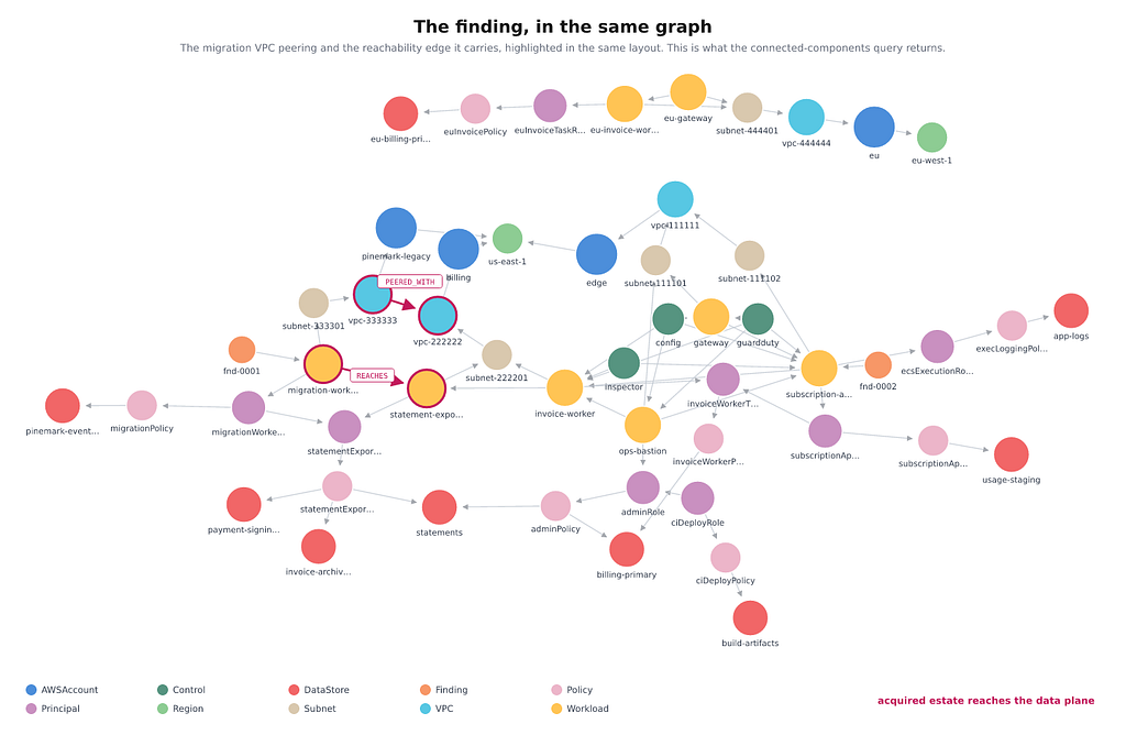
Plenty of estates are meant to be flat, so a single component is a failure only in context. It is one here because pinemark-legacy sits outside the audit boundary. The EU workloads form their own separate component, which the size(scopes) > 1 filter drops because every account in it shares the same scope.

For monitoring, compare component membership between snapshots. The count on its own is ambiguous, because a falling number can mean two groups became connected or simply that a component was deleted. Treat any change as a prompt to investigate.

Semantic search over the graph

Tagging is never as consistent as anybody wants, so an unclassified bucket is invisible to a query that filters on dataClass. Vector search gives a ranked shortlist of candidates instead.

The index stores one embedding per resource. Any property you want to filter on at search time has to be named in the WITH list when the index is created, which is why n.type appears there below.

CREATE VECTOR INDEX resourceEmb IF NOT EXISTS
FOR (n:AWSResource) ON (n.embedding) WITH [n.type]
OPTIONS { indexConfig: {
  `vector.dimensions`: 16,
  `vector.similarity_function`: 'cosine'
} };

Set vector.dimensions to whatever your embedding model produces. Embed something descriptive per resource, then search with the embedding of the question, here “historical customer invoice exports”:

MATCH (n:AWSResource)
SEARCH n IN (VECTOR INDEX resourceEmb FOR vector($queryVector, 16, FLOAT32)
             WHERE n.type = 's3' LIMIT 6) SCORE AS score
RETURN last(split(n.arn,':')) AS bucket, n.dataClass AS dataClass,
       round(score, 4) AS score ORDER BY score DESC;

bucket,                          dataClass,      score
"halyard-invoice-archive-2023",  "none",         0.9472
"halyard-statements",            "customer-pii", 0.875
"pinemark-events-raw",           "none",         0.6021
"halyard-build-artifacts",       "none",         0.5
"halyard-app-logs",              "operational",  0.5
"halyard-usage-staging",         "none",         0.5

Read the top two rows together. halyard-statements is already classified as customer data, so it landing second is the control that tells you the search works. The bucket above it is classified as nothing at all, and it holds invoice history.

That answers a question the reachability query raised, which is where dataClass comes from. AWS does not report it, and nothing infers it. The collector merges two independent sources. One is a classification tag your own people set. The other is Amazon Macie, the AWS service that scans S3 objects for sensitive data such as card numbers and credentials. Macie writes no tags of its own. It emits findings whose classificationDetails.result names the categories it detected, and the collector reads those findings.

The two sources can disagree. A bucket tagged internal that Macie reports as holding card numbers is a finding by itself, so store which source set the value and keep both. Anything neither covers is none, meaning unclassified rather than empty, which is what this search is for. A human confirms the shortlist and the reviewed value goes back for the evidence queries. Treat the ranking as triage, because an auditor will not accept “the embedding said so”.

Drift and snapshots

AWS remains the source of truth, so what matters is the change between last night’s collection and tonight’s. Each run writes one immutable ResourceState per resource and an EvidenceSnapshot pointing at that set, and comparing two snapshots gives new, changed, and disappeared fingerprints.

MATCH (prev:EvidenceSnapshot {snapshotId: $prevId})-[:OBSERVED]->(ps:ResourceState)
      -[:STATE_OF]->(r:AWSResource)
OPTIONAL MATCH (cur:EvidenceSnapshot {snapshotId: $curId})-[:OBSERVED]->(cs:ResourceState)
      -[:STATE_OF]->(r)
WITH r, ps, cs
WHERE cs IS NULL OR cs.fingerprint <> ps.fingerprint
RETURN r.arn AS resource,
       CASE WHEN cs IS NULL THEN 'deleted' ELSE 'modified' END AS change
UNION
MATCH (cur:EvidenceSnapshot {snapshotId: $curId})-[:OBSERVED]->(cs:ResourceState)
      -[:STATE_OF]->(r:AWSResource)
WHERE NOT EXISTS {
  (:EvidenceSnapshot {snapshotId: $prevId})-[:OBSERVED]->(:ResourceState)-[:STATE_OF]->(r)
}
RETURN r.arn AS resource, 'created' AS change;

resource,                                                            change
"...:loadbalancer/app/gateway/123456",                               "modified"
"arn:aws:s3:::halyard-build-artifacts",                              "deleted"
"arn:aws:lambda:us-east-1:222222222222:function:statement-export",   "created"

The subscription API sits in both snapshots and is absent from the result. Its fingerprint did not change, so it never reaches the diff.

The second branch of the UNION catches creations. Anchoring on the previous snapshot finds what changed or disappeared, but a resource existing only in tonight’s run has nothing to anchor to.

Compute the fingerprint in the collector, not in Cypher. The collector holds the raw Config JSON and can hash it with sorted keys, whereas hashing a property map inside the database means re-serialising something Neo4j gives no ordering guarantee for.

The agent that remembers

An agent that re-derives the same conclusion every night burns time and tells you nothing new. The state worth keeping is what changed, what was investigated, and what somebody accepted as an exception, none of which belongs in a graph rebuilt nightly. Neo4j’s Agent Memory Service is a hosted, graph-native place to keep it, and the two stores divide cleanly.

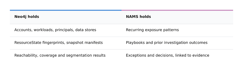
The link is by reference only. A remembered exception carries a resourceArn and a snapshotId that resolve in Neo4j but are plain strings in memory, so no estate data is duplicated. Resolution keyed on the ARN merges a bare identifier from one session with a fuller one from another.

NAMS keeps this material across nightly rebuilds. One part is the verdict, which in this case is that the migration peering was raised, ticketed as SEC-1042, and accepted until the migration ends. The route to that verdict is another, since the queries that confirmed a finding and the ones that cleared it carry more information than the conclusion alone. Over a longer period, repeated flags condense into a pattern.

When the peering was first raised somebody ran the one-hop reachability query, checked whether the target held customer data, and read the classification tag before deciding. Recording those steps turns a verdict into a playbook the next run can follow against tonight’s snapshot. The same shape on a different resource then starts from that recorded route.

Condensing is a separate job, run by a worker that folds repeated observations into a reflection superseding the ones it summarises. Forty-seven identical nightly flags become one line saying this path is always accepted. That line records how the path has been treated, which is a different claim from whether it is exploitable.

A stored exception suppresses nothing on its own. Your own logic checks expiresOn against today, and a fingerprint that moved since the accepted snapshot re-opens the finding instead of inheriting its verdict. NAMS stores the judgement and the working without making either. Interactive agents reach it over MCP, and unattended jobs post to the same REST API.

What this does not do

These limitations run in rough order of how often they matter. The queries identify candidates for review, since REACHES describes network exposure and GRANTS what a policy document says. Confirming that a path is usable takes IAM policy evaluation on top.

It is nightly, so between collections you are looking at history, and anything created and destroyed inside one window is invisible. The collector role is its own concern, because organisation-wide read across every account is a high-value target sitting in the graph it secures.

Do not infer feature availability from an Aura version string. An instance reporting a kernel of 5.27-aura still runs uuid(), string interpolation, SEARCH, ACYCLIC, and the native VECTOR type. Check the cheat sheet for your tier.

What to do next

Narrow the staleness window. Config emits configuration item changes to EventBridge, so changed resources can be updated as they change while the nightly run still writes the snapshots. The evidence chain stays intact and the graph stops lagging a day behind.

Model more of the network. Transit gateways, VPC endpoints, PrivateLink, and cross-region peering all move traffic this schema cannot see. Each one you add should move the component count, and if it does not, either your estate really is flat or your collector is dropping edges. Track that count per snapshot, alongside uncovered workloads and unclassified stores.

Give findings an owner. Link each resource back to the Terraform module that created it. An ARN gives you something to investigate, while a module path gives you a team and a pull request, which is usually what decides whether the finding gets fixed.

---

Auditing AWS infrastructure with Neo4j: questions inventory cannot answer was originally published in Neo4j Developer Blog on Medium, where people are continuing the conversation by highlighting and responding to this story.