Build a Semantic Layer from GCP with Neocarta

Consulting Engineer, Neo4j
14 min read

Build a graph-based semantic layer from GCP with Neocarta
Use Neocarta to easily build semantic layer graphs for your agentic applications in Neo4j
Introduction
Semantic layers are increasingly becoming an invaluable asset to agentic systems. They help an AI better understand the underlying data and enable it to handle large enterprise data landscapes. The key attribute of the modern semantic layer is the relationships among the many disparate data assets. What term does a column name resolve to? Are there other columns that share this meaning, and how can they be used to unlock novel insights? An agent with access to a graph-backed semantic layer has no problem connecting the dots and understanding where to find the answers in an ocean of data.
In this article, we will walk through how to use the Neocarta Python library to easily generate a semantic layer graph in Neo4j from information in GCP BigQuery and Knowledge Catalog (formerly Dataplex Universal Catalog). We will then use the Neocarta MCP server to allow an agent to gain immediate insights using the semantic layer.
Neocarta is a Neo4j Labs project and is undergoing rapid development.
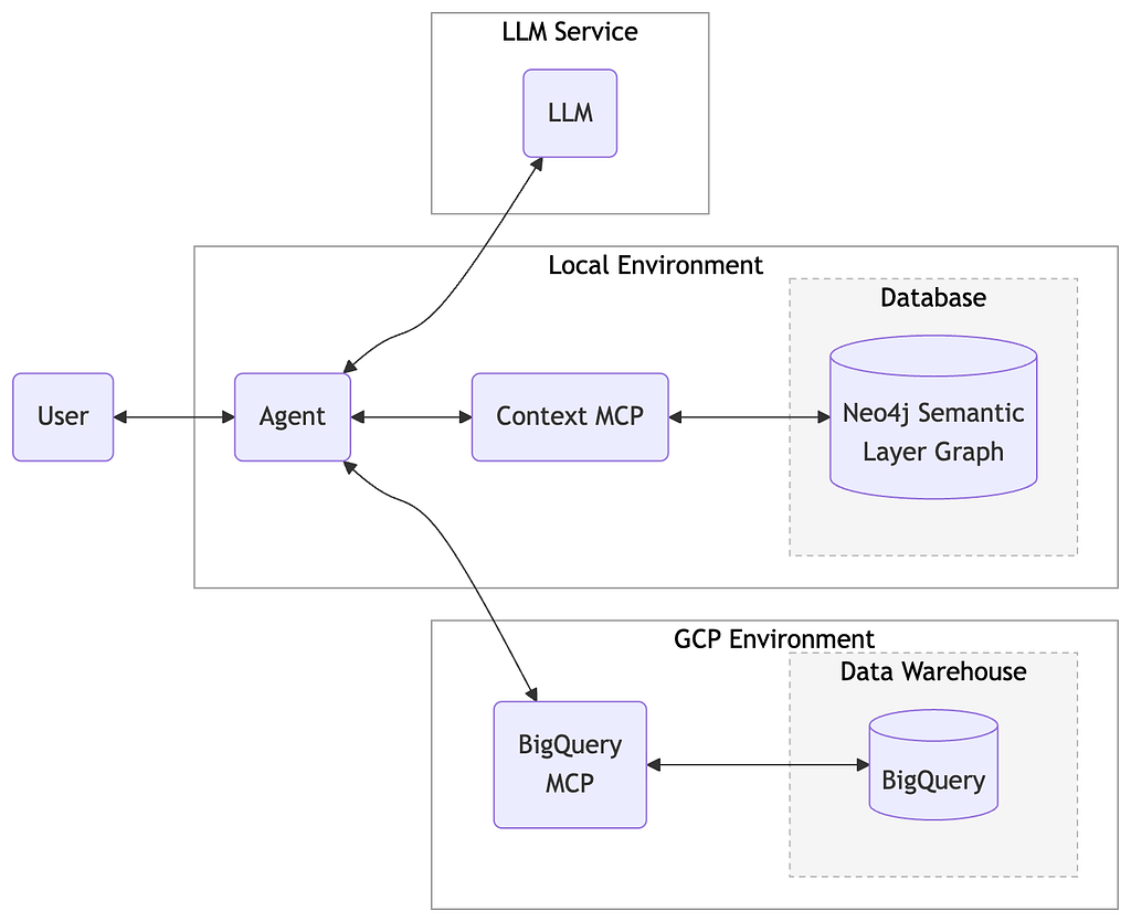
We will use the following semantic layer architecture as our template. Some aspects, such as the feedback and memory component, won’t be implemented in this walkthrough.
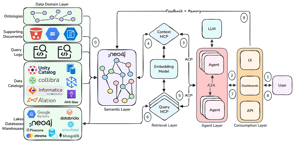
The semantic layer is first populated with source data in step 0. This includes a variety of data sources such as databases, data catalogs, query logs, supporting documents, and ontologies. This data provides the structure of the underlying data systems and facilitates understanding how to utilize it.
Once data is loaded, the user may interact with a resource in the consumption layer, such as a agentic chat interface. This will kick off an agentic workflow that first retrieves context from the Neo4j semantic layer via the context MCP server. The agents in the agent layer will then use this context to select the appropriate query MCP servers and execute queries against the source databases. The agent layer then summarizes the results and returns a response to the user.
Requirements
To run this demo end-to-end, you will need a few resources set up:
- GCP project with access to BigQuery and Knowledge Catalog (Dataplex Universal Catalog)
- gcloud CLI tool
- Neo4j instance — either local or Aura
- uv package manager installed
Graph Data Model
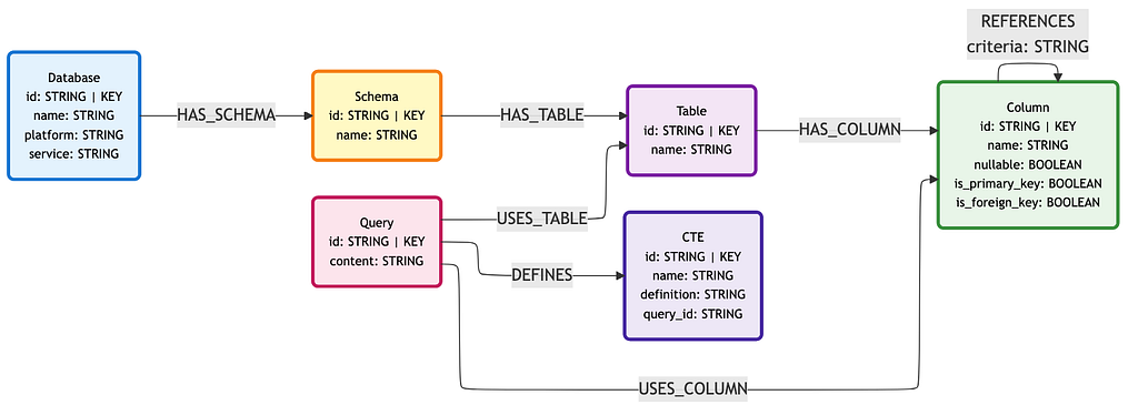
Before getting into the code, we should understand the shape of our semantic layer. There are two primary components we will implement (though we can include many more data sources; more on this in future articles).
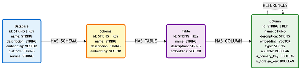
The foundation of our semantic layer is the metadata of our databases. Here, we explicitly map the database, schema, table, and column hierarchies in the graph. We also capture which columns relate to each other, either through foreign key definitions or by analyzing query patterns in the logs.
Note: Database maps to the GCP project, and Schema maps to a BigQuery dataset.
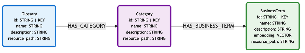
The second component is glossary information, which provides business terminology. These entities allow for more advanced search patterns when it comes to context retrieval.
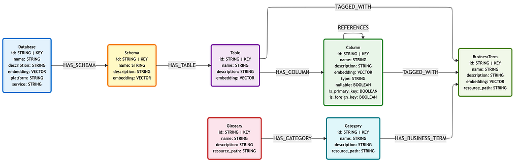
The glossary subgraph is layered over the metadata subgraph like so. BusinessTerm nodes are connected to Table and Column nodes via TAGGED_WITH relationships. This allows data assets to be identified via their connection to business terminology.
Data Sources
Our semantic layer will have two primary data sources: BigQuery and Knowledge Catalog. These will provide the schema metadata and glossary graph components, respectively.
We will also demonstrate how to import metadata from query logs. This augments the schema metadata graph with relationships that are not explicitly defined by foreign keys but can be instead inferred from JOIN conditions in SQL queries.
Below are the graph entities provided by each source.
BigQuery
- Database
- Schema
- Table
- Column
Knowledge Catalog (Dataplex)
- Glossary
- Category
- BusinessTerm
Query Logs
- Database
- Schema
- Table
- Column
- Query
- CTE
Neocarta includes connectors for BigQuery, Dataplex, and query logs, making it easy to generate this graph. It also supports other sources such as OSI YAML files.
Many other popular data source connectors are coming soon.
Creating The Graph
Now that we understand the graph data model and data sources for our semantic layer, we can begin building the graph.
We will be using one of the demo datasets in the Neocarta GitHub repository: the ACME Corp dataset. This data contains 33 tables, 327 columns, and 76 business terms.
First, clone the Neocarta GitHub repository. We will be locking this demo to Neocarta v0.7.0, so ensure you include the tag when cloning the repo.
git clone --branch neocarta-v0.7.0 https://github.com/neo4j-labs/neocarta.git
Navigate to the project root directory and open the .env.example file. We will need to create a new .env file based on the contents here.
Note: EMBEDDING_DIMENSIONS is not in the .env.example file. You may optionally add this variable to use non-default dimension values for models that support it. This applies to the Neocarta MCP server configuration. Configuration for the CLI is detailed further on.
NEO4J_USERNAME=neo4j-username
NEO4J_PASSWORD=neo4j-password
NEO4J_URI=neo4j-uri
NEO4J_DATABASE=neo4j-database
GCP_PROJECT_ID=project-id
GCP_PROJECT_NUMBER=project-number
BIGQUERY_DATASET_ID=acme_corp
BIGQUERY_LOCATION=us
DATAPLEX_LOCATION=us
DATAPLEX_GLOSSARY_ID=acme-corp-glossary
# Text2SQL agent chat LLM - LiteLLM model id. Examples:
# gpt-4o-mini
# gemini-2.0-flash
# gpt-5.4-mini
AGENT_MODEL=gpt-5.4-mini
# Embeddings - LiteLLM model id.
# Examples:
# text-embedding-3-small (OpenAI)
# gemini-embedding-001 (Vertex AI)
EMBEDDING_MODEL=text-embedding-3-small
# EMBEDDING_DIMENSIONS=768
# Provider credentials - set the variables your chosen EMBEDDING_MODEL requires.
OPENAI_API_KEY=…
# GEMINI_API_KEY=…
Note: The AGENT_MODEL environment variable is only relevant if you decide to use the built-in CLI agent. It is preferred to use an agentic application such as Claude Desktop for the agent interface.
Note: Neocarta is compatible with any embedding models supported by LiteLLM.
Once you have created a .env file in the project root, run the following to install the core project and CLI dependencies:
uv sync --extra cli
You also need to sign in to the gcloud CLI in order to connect to your GCP instance.
gcloud auth application-default login
Now we can populate our BigQuery database and Knowledge Catalog glossary with the demo data (You may skip this step if you already have data to use).
First, populate BigQuery.
uv run datasets/load_bigquery.py --dataset acme
Now we can populate the Knowledge Catalog glossary data.
Note: All references to Knowledge Catalog in Neocarta are named Dataplex.
The command below will generate the glossary.
datasets/dataplex/create_acme_glossary.sh
This command links business terms to their respective data assets.
uv run datasets/dataplex/connect_acme_terms.py
Now that our GCP project is populated with data, we can create our semantic layer in Neo4j. This will be done using the Neocarta CLI. Since we are in the Neocarta project, we don’t need to install the CLI; however, in other circumstances, you may install the CLI from PyPI.
pip install "neocarta[cli]"
# or
uv add "neocarta[cli]"
Ensure that your Neo4j instance is running, and then execute the following two CLI commands. Both of these commands will ingest data and generate embeddings for the default node sets (Table and Column for the schema, and BusinessTerm for the glossary).
Note: We are using uv run here because uv manages the Neocarta environment. A global install may be run without the uv run prefix.
You may also use the –embedding-dimensions flag to define the embedding dimensions to use if the model supports it. This applies to both CLI commands.
uv run neocarta bigquery schema --embeddings
By running the Knowledge Catalog (Dataplex) connector second, we ensure that business terms will be connected to the existing schema components via TAGGED_WITH relationships.
uv run neocarta dataplex glossary --embeddings
Now we can enhance the relationships between our data assets in the semantic layer by parsing query logs as well. This can add additional JOIN logic between tables and columns that isn’t captured in the foreign key definitions. Since we don’t have any query log data in our fresh demo dataset, we won’t run this section. Feel free to run it on your existing BigQuery datasets.
Note: The query log connector will also store Query and CTE nodes in our semantic layer. These may be referenced as few-shot examples.
Run the below CLI command to connect to the BigQuery query logs and ingest into the Neo4j semantic layer graph. Feel free to replace the start date flag with your desired date. See the CLI documentation for more details on configuration.
uv run neocarta bigquery logs --start-date 2026–01–01
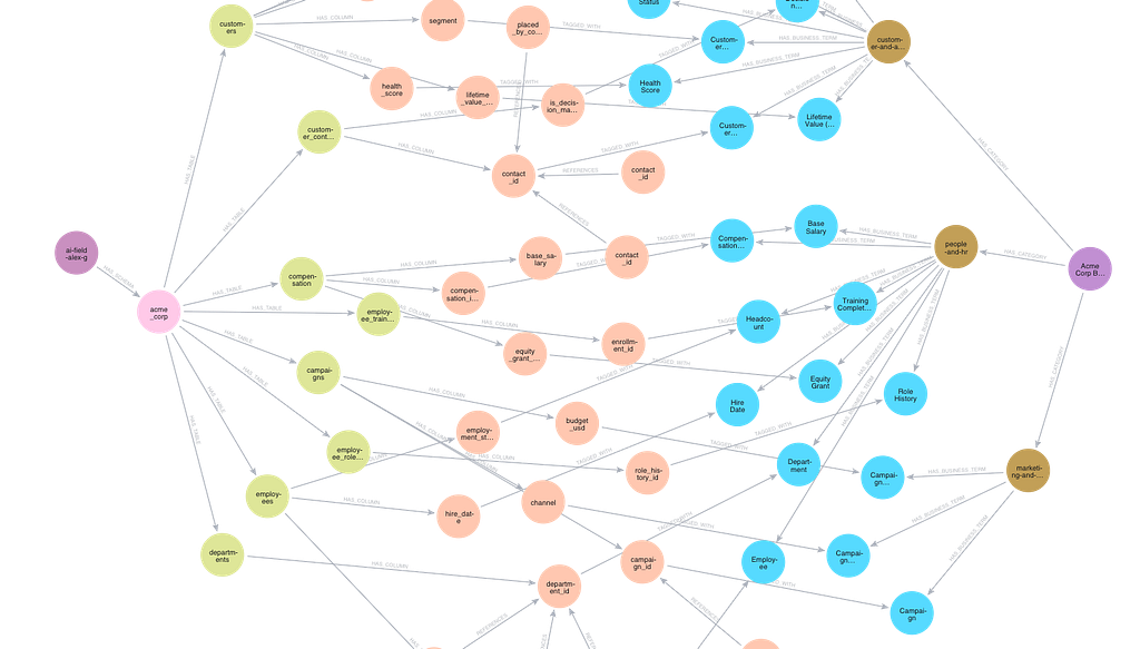
Here is a snapshot of the resulting semantic layer graph. The left side contains the Database (dark purple) → Schema (pink) → Table (yellow green) → Column (orange) hierarchy, and the right side contains Glossary (dark purple) → Category (brown) → BusinessTerm (blue).
Wiring an Agent to The Semantic Layer
Now it’s time to connect an agent to our semantic layer graph. This is easily done with the Neocarta MCP server. This MCP server is built to be compatible with the graph data model defined in Neocarta and will register tooling according to the indexes and entities available in the graph.
Since we have vector indexes, full-text indexes, and BusinessTerm nodes in our graph, the MCP server will register the following toolset:
- List schemas
- List tables by schema
- Get context by table business term hybrid search
- Get context by column business term hybrid search
- Get full metadata schema (Only used for development and debugging)
Note: Full-text indexes are automatically generated for name and description properties, but can be turned off in the Python library connector arguments.
The two hybrid search plus business term tools feature the most advanced context retrieval patterns. They will perform three searches to first identify the anchor node pool:
- Primary entity vector search
- BusinessTerm full-text search
- Primary entity full-text search
The full-text search portion first identifies BusinessTerm nodes, then traverses to connected entity nodes (either Table or Column). Full-text search is then run again on these entity nodes, and the normalized average score is calculated. These results are then combined with the vector search results, ranked by score, and filtered to the top k.
The easiest way to test the semantic layer is by using the built-in CLI agent in the Neocarta repository. You will need to ensure that your embedding model API key is included in the valid environment variables list in the run_agent.py file. You will also need to install the optional MCP and agent dependencies.
uv sync --all-groups
In addition, you will also need to enable the remote BigQuery MCP server:
gcloud beta services mcp enable bigquery.googleapis.com --project=PROJECT_ID
And locally authenticate via the gcloud CLI:
gcloud auth application-default login
Then run the following command from your command line:
make agent
This will spin up a local LangGraph agent, the Neocarta MCP server, and connect to the BigQuery remote MCP server.
Alternatively, you may connect any MCP application to the semantic layer we created by adding the Neocarta MCP server to your MCP configuration. Below is an example of a Claude Desktop configuration JSON with the Neocarta and BigQuery MCP servers. If using this method, you should also disable schema retrieval tooling for the BigQuery MCP server. You will only need the execute_sql tool.
Note: This configuration is using the BigQuery MCP server from the Google toolbox-sdk, not the remote BigQuery MCP server. This makes it easier to handle auth configuration.
{
  "mcpServers": {
    "neocarta": {
      "command": "uvx",
      "args": [
        "--from",
        "neocarta[mcp]@0.7.0",
        "neocarta-mcp"
      ],
      "env": {
        "NEO4J_URI": "neo4j+s://xxxxxxxx.databases.neo4j.io",
        "NEO4J_USERNAME": "neo4j",
        "NEO4J_PASSWORD": "your-password",
        "NEO4J_DATABASE": "neo4j",
        "OPENAI_API_KEY": "sk-...",
        "EMBEDDING_MODEL": "text-embedding-3-small",
        "EMBEDDING_DIMENSIONS": "768"
      }
    },
    "bigquery": {
      "command": "npx",
      "args": ["-y", "@toolbox-sdk/server", "--prebuilt", "bigquery", "--stdio"],
      "env": {
        "BIGQUERY_PROJECT": "your-gcp-project-id"
      }
    }
  }
}
Asking Questions
We now have the agent connected to our semantic layer and BigQuery instance via MCP and can begin analyzing our data.
Note: These responses were generated with OpenAI gpt-4o-mini
We can start with an easy question:
Which product line contributes the most to total ARR, and what is the breakdown?
This should utilize the subscription and products tables, with the result looking something like the table and summary below.
SELECT
  p.name                                                        AS product,
  COUNT(s.subscription_id)                                      AS active_subscriptions,
  SUM(s.arr_usd)                                                AS arr_usd,
  ROUND(SUM(s.arr_usd) / SUM(SUM(s.arr_usd)) OVER () * 100, 1) AS pct_of_total
FROM acme_corp.subscriptions s
JOIN acme_corp.products p ON s.product_id = p.product_id
WHERE s.status = 'active'
GROUP BY p.name
ORDER BY arr_usd DESC
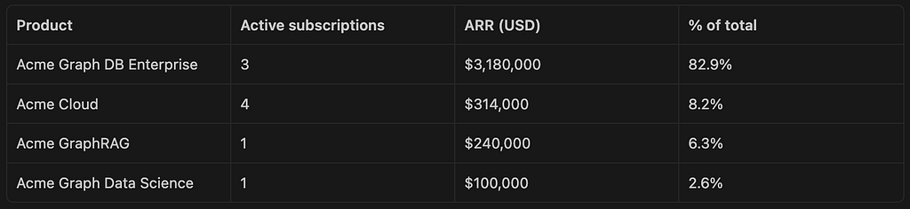
“Graph DB Enterprise is the dominant revenue driver, accounting for over 80% of ARR despite having fewer subscriptions than Cloud. This concentration in a single product line is a key business risk to monitor.”
Now let’s ask a slightly more difficult question:
How are performance ratings distributed across departments in the most recent review cycle?
This requires three tables: performance_reviews, employees, and departments, and the results should resemble the following insights. Note that the most recent data is from late 2024.
SELECT
  d.name           AS department,
  pr.overall_rating,
  COUNT(*)         AS employees,
  ROUND(AVG(pr.numeric_score), 2) AS avg_score
FROM acme_corp.performance_reviews pr
JOIN acme_corp.employees e  ON pr.employee_id  = e.employee_id
JOIN acme_corp.departments d ON e.department_id = d.department_id
WHERE pr.review_period = '2024-H2'
GROUP BY d.name, pr.overall_rating
ORDER BY d.name, pr.overall_rating
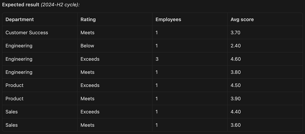
“Engineering has the widest performance spread — three “Exceeds” employees averaging 4.6, alongside one “Below” employee at 2.4. Sales and Product skew positive. Customer Success has only one reviewed employee, suggesting a data coverage gap to investigate.”
Now, a question that requires calculating some scores and inferring information about the situation.
Is there a correlation between a customer’s health score and their support experience?
This should join two tables: customers and support_tickets, and have results resembling the following insights.
SELECT
  c.company_name                                              AS customer,
  c.segment,
  c.health_score,
  c.status                                                    AS account_status,
  COUNT(t.ticket_id)                                          AS total_tickets,
  ROUND(AVG(t.csat_score), 1)                                 AS avg_csat,
  ROUND(AVG(TIMESTAMP_DIFF(t.resolved_at, t.created_at, HOUR)), 1) AS avg_resolution_hrs
FROM acme_corp.customers c
LEFT JOIN acme_corp.support_tickets t ON c.customer_id = t.customer_id
GROUP BY c.company_name, c.segment, c.health_score, c.status
ORDER BY c.health_score ASC
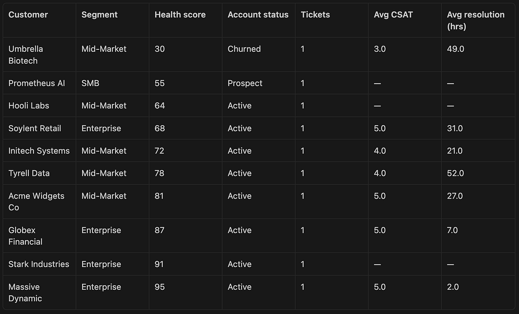
“A clear positive correlation emerges between health score and support quality. The churned customer (Umbrella Biotech, score 30) had the lowest CSAT (3.0) and the longest resolution time (49 hrs) of any rated ticket. Conversely, the two highest-scoring customers — Massive Dynamic (95) and Globex Financial (87) — had perfect CSAT scores and the fastest resolution times (2 hrs and 7 hrs respectively). This suggests that support responsiveness is both a leading indicator of and contributor to customer health. Customers with CSAT scores below 4.0 or resolution times above 30 hours warrant proactive CSM outreach.”
Summary
In this walkthrough, we demonstrated how to build a semantic layer in Neo4j using the Neocarta Python library. We integrated BigQuery schema metadata and Knowledge Catalog glossary information to create a rich, traversable map of our data landscape. This allowed the agent to answer increasingly complex questions about our data while keeping the context light.
If you encountered any issues while using Neocarta or have ideas for features, please raise a GitHub issue on the repository’s Issues page.
Build a Semantic Layer from GCP with Neocarta was originally published in Neo4j Developer Blog on Medium, where people are continuing the conversation by highlighting and responding to this story.
Share Article


Explore
Related Articles

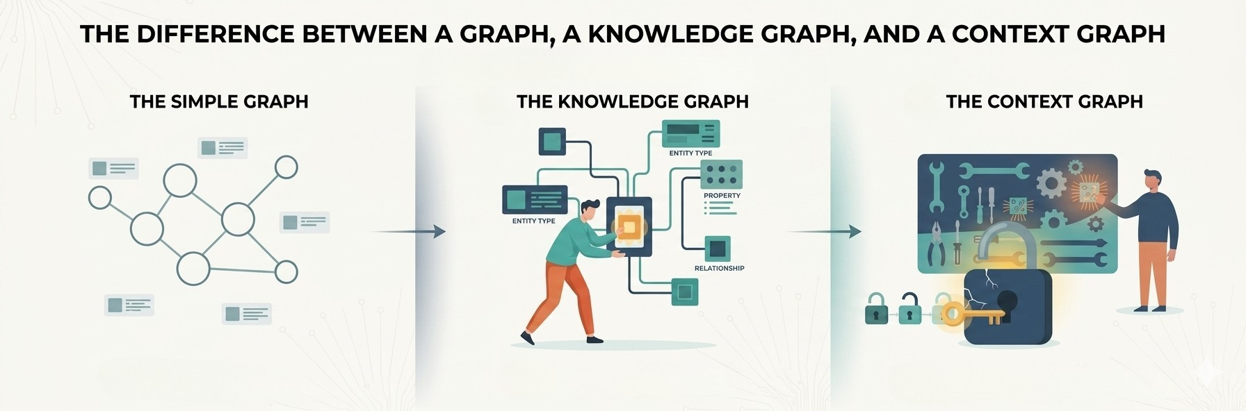
1 of 3: The difference between a graph, a knowledge graph, and a context graph
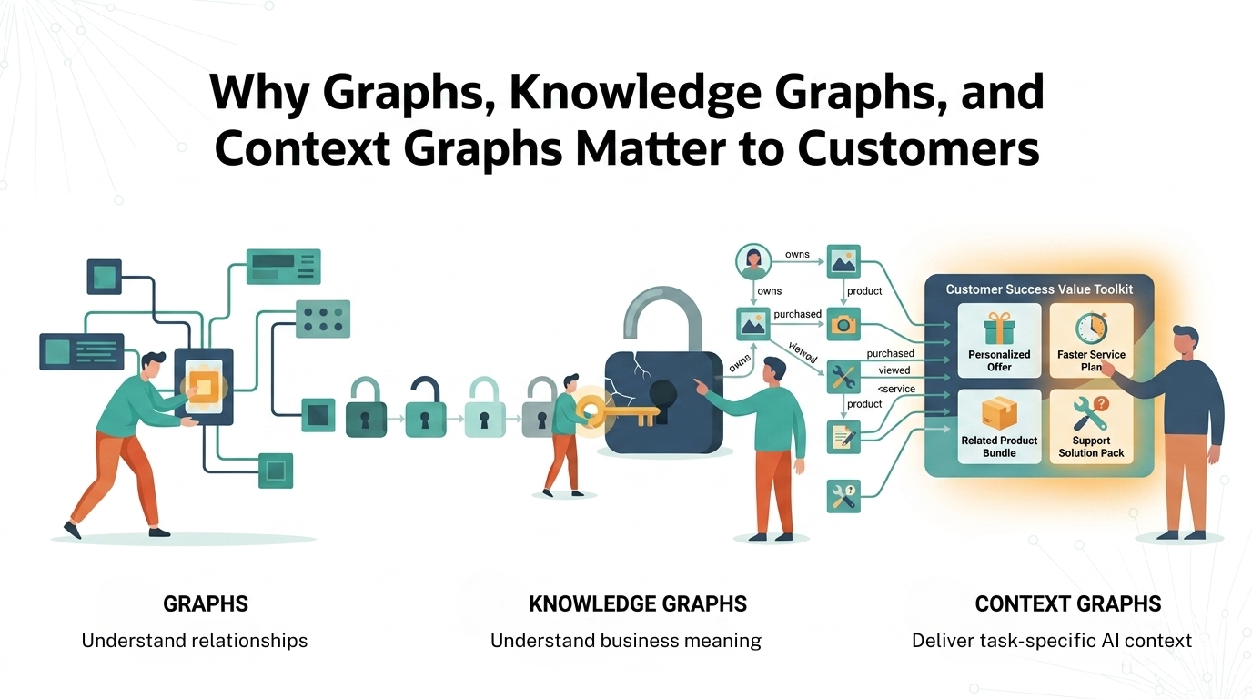
2 of 3: Why graphs, knowledge graphs, and context graphs matter to customers
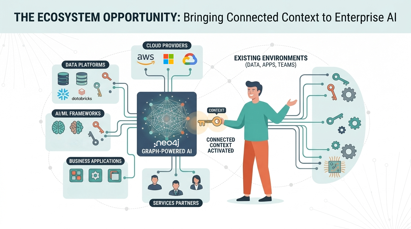
3 of 3: The graph ecosystem: Bringing connected context to enterprise AI
Digital twins that learn: connected asset intelligence with Neo4j and Databricks