Seeds of Science, Visuals in Bloom: Introudcing Whole-Graph Projections

Bloom, part of Neo4j’s suite of user tools, has offered analysts the ability to run a selection of Data Science algorithms for quite a while. There has, however, been a major caveat — until now, algorithms could only be run on the graph in the current Bloom Scene, giving a local view of communities or centrality measures. With our most recent updates, there’s also an option to configure & run a graph algorithm across the entire database from Bloom.

How can graph algorithms be of use?

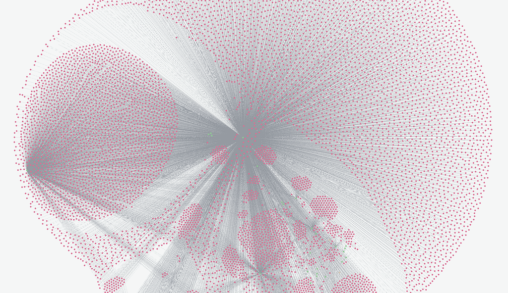
Graph algorithms are a powerful way to unlock insights from data. Centrality algorithms can help identify nodes of high importance, bottlenecks or chokepoints, for example. Meanwhile, community detection algorithms can highlight groups of nodes that are more closely connected. Graph visualizations are a fantastic way to make graph algorithms come alive.

Bloom provides not only a no-code way to configure and run algorithms, but also an easy way to highlight results with rule-based styling. You can apply graph algorithms either on data in a Scene (as before), or, now, by creating a projection across the entire database, all from the Bloom user interface.

Why offer two options?

Graph algorithms are run on a projection, which can be thought of as a temporary copy of the structure of a certain subset of data in the graph. For example, a projection might involve all nodes with the label Ingredient or Recipe, and all relationships of the type Uses. Even though the database might have many other labels and relationship types, we might be interested in discovering only which ingredients are most used across all known recipes.

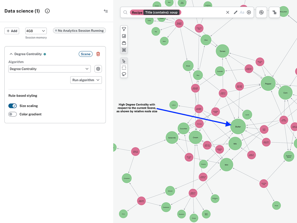
A Bloom Scene can define the projection for running a graph algorithm. For example, we might only be interested in learning which ingredients are most commonly used in recipes for soup. In that case, we could create a Bloom Scene with only that data, and choose to run a degree centrality algorithm (degree centrality will count the number of relationships connecting to each node). Perhaps we’d find that butter is one of the most used ingredients for soups. Running algorithms on the local Scene also provides a quick way to try out different algorithms and see how they highlight different aspects of your data in a fully contained view, with the added bonus of not adding properties with results back to the database. It can be a good proving ground, a way to look at just local parts of the graph, or a way to learn how different algorithms work.

On the other hand, we might want to calculate the degree centrality for all ingredient & recipe nodes across the entire database, and bring up subsets to look at ad-hoc. In this case we could apply the new whole-graph algorithm capability in Bloom, and each time we populate a Bloom Scene we’d have the degree centrality measure on each node, based on a calculation run across the entire relevant data set. In this case we might find that milk is less well-connected compared to an ingredient like pepper, when looking at the whole data set. In the image below we can see that the “Degree Centrality” for pepper, when measured with just our Scene data for soup, is 6. Looking at “Degree Centrality 1”, we see that pepper is actually connected to more than 16000 recipes in the entire underlying data set.

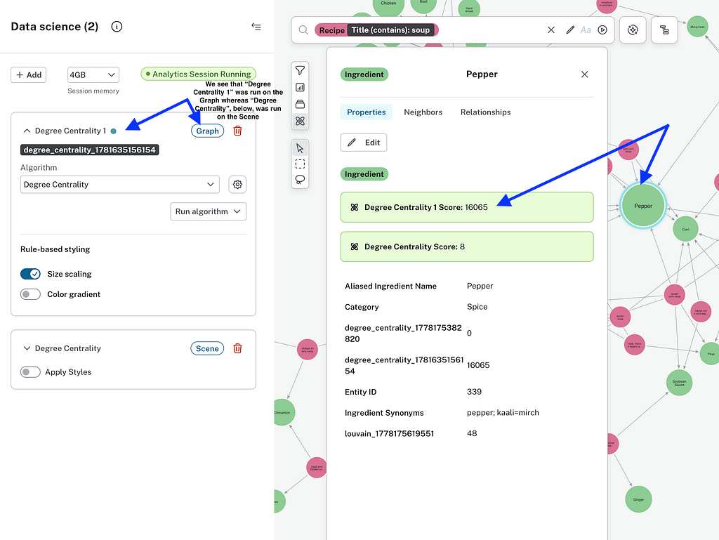
In the former case, we’re limiting graph algorithm calculations to the specific local scene of interest and we’re not writing results back to the database — they are available only in the Scene for the elements that are included there. In the latter case we take into account all relevant data in the database even if it’s not currently visualized on the scene, and write the result back to the graph for future reference.

Getting started — how to run algorithms on your graph with Bloom

As mentioned above, with recent updates we’ve introduced the ability to configure and run graph algorithms on a projection based on your entire database, as an alternative to just the data in the current Scene. This capability is available for Neo4j Instances using either the Graph Data Science (GDS) plugin or the Aura Graph Analytics (AGA) service. All of this can be done without writing any code, all from the Bloom user interface.

To get started, load Bloom either from the Aura console, or a standalone or Desktop installation. If the connected instance has Data Science capability (either via the GDS plugin or AGA), you’ll find the Data Science icon on the left side of the screen just under the search bar.

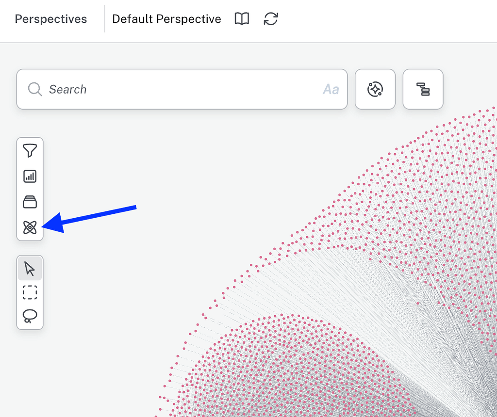
From here, you can choose from a selection of algorithms that are well suited to visualizing results — namely some centrality and community detection algorithms. Once you’ve chosen an algorithm, you can optionally define additional configuration settings like which labels and relationship types the algorithm should consider, and any properties to use for weighting, as well as directionality.

Finally, there are now two options under the ‘Run algorithm’ button: ‘Apply to current scene’ will run the algorithm on only the data in the current Bloom scene, and store the results with the scene (but not write results back to the database). The second option is new, ‘Create projection on the entire graph’. This will use all of the data in your database to build a projection based on the setting selected, and run the algorithm across this entire data set. In this case, results are written to the database in the Property chosen at run time so they can be referenced later.

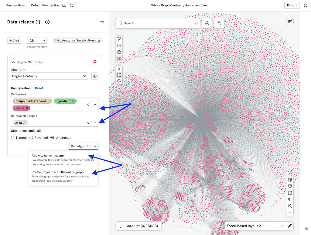
With either option, Bloom allows you to automatically apply colour and/or size styling to the scene based on the algorithm’s output. Of course, output will be different for an algorithm run on the local scene only, vs on the entire graph, because in the latter case there are additional parts of the graph that aren’t visible on-scene, and these will influence any data science results. Changes to the database or scene won’t automatically be reflected in results, either, so algorithms will need to be re-run to capture any changes in results due to changes in data. Note that it is possible, using the GDS Python client or the Cypher API, to schedule automatic runs of data science algorithms. While this falls outside the scope of Bloom’s no-code capabilities for data science, analysts can use Bloom to fine tune their algorithms and later schedule them outside Bloom.

Final thoughts

As Neo4j’s low/no-code graph exploration tool, Bloom is found in the Aura Console (previously known as Explore in the Console) and the Neo4j Enterprise Studio for self-managed installations. It’s also available in Neo4j Desktop.

Neo4j’s data science capabilities can be a highly useful way to derive insights from data, and there’s a great deal of capability beyond the functionality exposed by the Bloom user interface.

You can find documentation for both Bloom’s graph analytics capabilities as well as the data science capabilities in general and Aura Graph Analytics online.

Give it a try, and see what you can learn!

Seeds of Science, Visuals in Bloom: Introudcing Whole-Graph Projections was originally published in Neo4j Developer Blog on Medium, where people are continuing the conversation by highlighting and responding to this story.