Deep Dive: Neo4j Virtual Graph on BigQuery

Neo4j Virtual Graph on BigQuery

Query and visualise BigQuery data as if it were in Neo4j

I have always wanted a Porsche. It looks good, it is comfortable and it is fast. Now, the speed isn’t that important, I am not allowed to drive faster than 120 km/h anyway… unless I go down to Germany and drive on the Autobahn. But even then I am not much for driving fast, I am more for the comfort and the looks. So if someone said they could pimp up my old SAAB with the looks and comfort of a Porsche, without having to buy a new car, I would definitely go for it.

In my metaphor the SAAB is BigQuery and Neo4j is the Porsche. I know, that’s quite unfair and not a little arrogant. When it comes to searching large quantities of data, few things are as fast as BigQuery. But bear with me for the point I try to make (and honestly, being compared to a SAAB 99 might be the best compliment one could get from a Swede).

What database paradigm that would be the SAAB and which would be the Porsche depends on the use case of course. There are use cases where the tabular model is superior, and there are those that fit best for document databases, but what we focus on here are the “graphy” use cases and that is where Neo4j is the Porsche.

And when we say that you benefit from a graph database for “graphy” use cases it actually means three different things; three different benefits you get:

1. Graph Query languages are better at expressing those types of queries (The Comfort)
2. The visual graph is better at showing that type of data (The Looks)
3. It is faster at traversing those relationships because of the native graph and its “index-free adjacency” structure (The Speed)

Neo4j Virtual Graphs

In June 2026, Neo4j released a preview of a new capability called Virtual Graphs, which allows you to create a virtual Neo4j instance that acts as a wrapper over a relational data store such as BigQuery, Databricks or Snowflake, and let you run Cypher queries, GDS Algorithms and all the Neo4j tools on that data as if it were a graph. And this is done with zero ETL, the data remains in the relational data store.

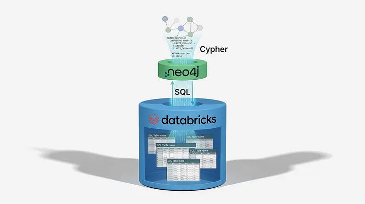
This solves items number 1 and 2 above. It allows you to express your graph questions with Cypher/GQL and it can visualise the result as a graph. It will, however, not solve the execution time, as it is still the same relational engine underneath. But maybe you don’t have any real-time requirements, and maybe it is ok for the query to take time?

This is the Porsche analogy. Except that in this case it doesn’t look like a duct tape fixed-up SAAB, but it has the looks and comfort of the real thing, just with the SAAB engine under the hood (and not in the trunk as on the Porsche 911).

I will now take you through Neo4j Virtual Graphs on top of BigQuery with a simple use case, but a fairly large data set.

The Data

“Oh no, not yet another movie graph”

Yes, sorry, it will be another movie graph. But an interesting movie graph as it will contain all movies and TV series ever made, as well as all actors and other crew members, since we will take the data directly from the IMDB (Internet Movie DataBase) public data set. This way we can easily get a dataset with over a hundred million rows that anyone can recreate with a simple query.

I promise I will have another, maybe more real-world, use case for my next blog 🙂

Here is how you get this data up and running on BigQuery in 5 minutes (plus the time to transfer files):

Download the 7 g-zipped TSV (Tab Separated) files from the link on the IMDB page above.

1. Create a Project in the Google Cloud Console, if you don’t already have one.
2. Create a bucket in Google Cloud Storage for this project and upload the files there (you don’t have to unzip them).
3. Go to BigQuery and run the query below. It takes about 5 minutes to run, and then you have a table with ~15.4 million persons (actors, directors and other crew), ~12.6 million titles (movies, TV series, episodes, video games etc.) and ~99.9 million relationships between the persons and the titles.

-- ==========================================
-- 1. INITIALIZE SCHEMA
-- ==========================================
CREATE SCHEMA IF NOT EXISTS imdb;

-- ==========================================
-- 2. CREATE AND LOAD: NAMES
-- ==========================================
-- Step A: Load into a temporary staging table
LOAD DATA OVERWRITE imdb.staging_names (
    nconst STRING,
    primaryName STRING,
    birthYear STRING,
    deathYear STRING,
    primaryProfession STRING,
    knownForTitles STRING
)
FROM FILES (
  format = 'CSV',
  field_delimiter = '\t',
  skip_leading_rows = 1,
  null_marker = '\\N',
  quote = '',                    
  allow_jagged_rows = true,      
  ignore_unknown_values = true,  
  uris = ['gs://[BUCKETNAME]/name.basics.tsv.gz']
);

-- Step B: Transform and load into final production table
CREATE OR REPLACE TABLE imdb.names AS
SELECT
  CAST(REGEXP_REPLACE(nconst, r'^[a-zA-Z]{2}', '') AS INT64) AS nconst,
  primaryName,
  SAFE_CAST(birthYear AS INT64) AS birthYear,
  SAFE_CAST(deathYear AS INT64) AS deathYear,
  primaryProfession,
  knownForTitles
FROM imdb.staging_names;

ALTER TABLE imdb.names ADD PRIMARY KEY (nconst) NOT ENFORCED;


-- ==========================================
-- 3. LOAD RAW DATA INTO SEPARATE STAGING TABLES FOR TITLES
-- ==========================================

-- Staging Basics
LOAD DATA OVERWRITE imdb.staging_basics (
    tconst STRING,
    titleType STRING,
    primaryTitle STRING,
    originalTitle STRING,
    isAdult STRING,
    startYear STRING,
    endYear STRING,
    runtimeMinutes STRING,
    genres STRING
)
FROM FILES (
  format = 'CSV',
  field_delimiter = '\t',
  skip_leading_rows = 1,
  null_marker = '\\N',
  quote = '',
  allow_jagged_rows = true,
  ignore_unknown_values = true,
  uris = ['gs://[BUCKETNAME]/title.basics.tsv.gz']
);

-- Staging Ratings
LOAD DATA OVERWRITE imdb.staging_ratings (
    tconst STRING,
    averageRating STRING,
    numVotes STRING
)
FROM FILES (
  format = 'CSV',
  field_delimiter = '\t',
  skip_leading_rows = 1,
  null_marker = '\\N',
  quote = '',
  allow_jagged_rows = true,
  ignore_unknown_values = true,
  uris = ['gs://[BUCKETNAME]/title.ratings.tsv.gz']
);

-- Staging Episodes
LOAD DATA OVERWRITE imdb.staging_episodes (
    tconst STRING,
    parentTconst STRING,
    seasonNumber STRING,
    episodeNumber STRING
)
FROM FILES (
  format = 'CSV',
  field_delimiter = '\t',
  skip_leading_rows = 1,
  null_marker = '\\N',
  quote = '',
  allow_jagged_rows = true,
  ignore_unknown_values = true,
  uris = ['gs://[BUCKETNAME]/title.episode.tsv.gz']
);


-- ==========================================
-- 4. BUILD THE MASTER TITLES TABLE
-- ==========================================
CREATE OR REPLACE TABLE imdb.titles AS 
SELECT 
    CAST(REGEXP_REPLACE(b.tconst, r'^[a-zA-Z]{2}', '') AS INT64) AS tconst,
    b.titleType,
    b.primaryTitle,
    b.originalTitle,
    SAFE_CAST(b.isAdult AS BOOLEAN) AS isAdult,
    SAFE_CAST(b.startYear AS INT64) AS startYear,
    SAFE_CAST(b.endYear AS INT64) AS endYear,
    SAFE_CAST(b.runtimeMinutes AS INT64) AS runtimeMinutes,
    b.genres,
    SAFE_CAST(r.averageRating AS FLOAT64) AS averageRating,
    SAFE_CAST(r.numVotes AS INT64) AS numVotes,
    CAST(REGEXP_REPLACE(e.parentTconst, r'^[a-zA-Z]{2}', '') AS INT64) AS parentTconst,
    SAFE_CAST(e.seasonNumber AS INT64) AS seasonNumber,
    SAFE_CAST(e.episodeNumber AS INT64) AS episodeNumber
FROM imdb.staging_basics b
LEFT JOIN imdb.staging_ratings r ON b.tconst = r.tconst
LEFT JOIN imdb.staging_episodes e ON b.tconst = e.tconst;

ALTER TABLE imdb.titles ADD PRIMARY KEY (tconst) NOT ENFORCED;


-- ==========================================
-- 5. CREATE AND LOAD: PRINCIPALS
-- ==========================================
-- Step A: Load into temporary staging table
LOAD DATA OVERWRITE imdb.staging_principals (
    tconst STRING,
    ordering STRING,
    nconst STRING,
    category STRING,
    job STRING,
    characters STRING
)
FROM FILES (
  format = 'CSV',
  field_delimiter = '\t',
  skip_leading_rows = 1,
  null_marker = '\\N',
  quote = '',
  allow_jagged_rows = true,
  ignore_unknown_values = true,
  uris = ['gs://[BUCKETNAME]/title.principals.tsv.gz']
);

-- Step B: Transform, generate a unique row sequence, and build final table
CREATE OR REPLACE TABLE imdb.principals AS
SELECT
  ROW_NUMBER() OVER() AS id,
  CAST(REGEXP_REPLACE(tconst, r'^[a-zA-Z]{2}', '') AS INT64) AS tconst,
  SAFE_CAST(ordering AS INT64) AS ordering,
  CAST(REGEXP_REPLACE(nconst, r'^[a-zA-Z]{2}', '') AS INT64) AS nconst,
  category,
  job,
  characters
FROM
  imdb.staging_principals;

-- Apply constraints
ALTER TABLE imdb.principals ADD PRIMARY KEY (id) NOT ENFORCED;
ALTER TABLE imdb.principals ADD CONSTRAINT fk_principals_titles FOREIGN KEY (tconst) REFERENCES imdb.titles (tconst) NOT ENFORCED;
ALTER TABLE imdb.principals ADD CONSTRAINT fk_principals_names FOREIGN KEY (nconst) REFERENCES imdb.names (nconst) NOT ENFORCED;


-- ==========================================
-- 6. CLEAN UP ALL STAGING TABLES
-- ==========================================
DROP TABLE IF EXISTS imdb.staging_names;
DROP TABLE IF EXISTS imdb.staging_basics;
DROP TABLE IF EXISTS imdb.staging_ratings;
DROP TABLE IF EXISTS imdb.staging_episodes;
DROP TABLE IF EXISTS imdb.staging_principals;

We do a couple of things here. We import 5 of the TSV files into 3 tables (we combine ratings and episodes into the titles table), and we cast the datatypes from the strings in the TSV to what they should be. But we also do something with the IDs. The tconst and nconst keys are strings, but in fact they both start with two letters followed by just digits, so I just strip out the letters and convert the rest to a number. For the principals table I introduce a new id, which is just a sequential number (the row number in the TSV). Having integer keys isn’t necessary, we could have kept them as strings, but it will make our life easier when we get to the GDS part in a later chapter.

To be able to access this data from Neo4j you need to create an access key. Start by creating a service account (if you don’t already have one). Under your service account go to the Keys tab and select Add key->Create new key. The key type should be JSON. Download the generated JSON key file and keep it for later.

ETL vs non-ETL

Now we want to use this data as a graph, and through Neo4j we have two options:

• Importing the data to a native Neo4j instance (full ETL)
• Running Virtual Graph to project the data as a graph (no ETL)

From a surface level they both look the same. Both appear and behave as regular Neo4j instances and supports all regular Neo4j tools, drivers and Cypher queries*, but under the hood they are very different. We will do both and make some comparisons.

* There are some limitations to the Cypher support in Virtual Graph

Data model

For both options you need to create a graph model that tells the system how the relational model should map to a graph. In the Neo4j Aura console you use the same tool, and the same graph model (as well as the same data source definitions) for both, which makes it very simple if you later decide that you want to go from a Virtual Graph to a full native instance.

So we will create a data source for our BigQuery instance and a graph model for our use case, and then we’ll create two instances, one native instance where we run an import job, and one Virtual Graph instance.

This is the data model of the BigQuery tables:

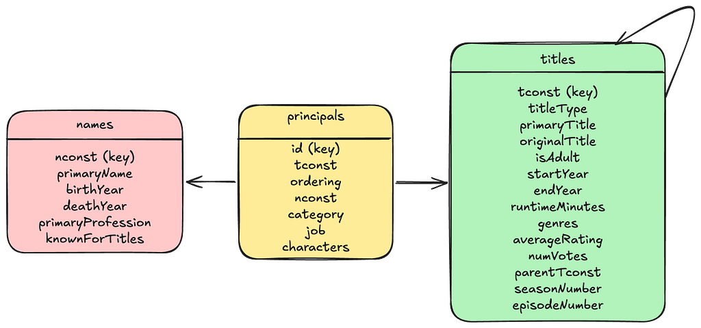
And this is how we want to have it modelled as a graph:

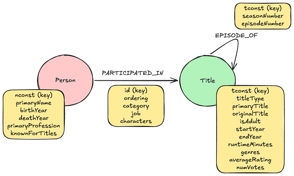
Creating our instances

Now let’s login to Aura and go to the Instances tab to create our two instances.

We’ll start with the native instance. Click Create instance and select the instance configuration you want. You can select any type, size, region etc. The only hard requirement is that the disk size is at least 64 GB to fit our imported graph. I will go with a Professional Instance on GCP with 48 GB RAM and 96 GB disk (to make sure that our full graph can fit in RAM). I gave mine the name BigQuery_IMDB_Import.

Wait for the instance to spin up and then switch over to the Import tab. Under the first tab, Data sources, click New Data Source. Select BigQuery and then fill in the credentials for your instance. In the Service Account Key JSON field you need to paste the full text content of the JSON key file you downloaded from BigQuery in the earlier chapter.

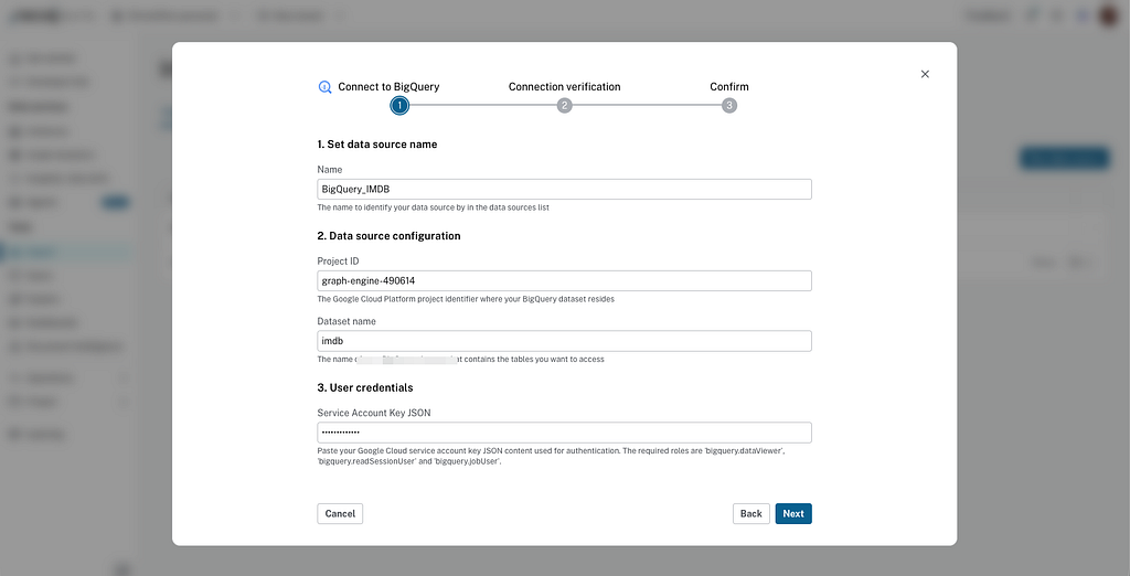
Click Next and it will validate your connection. Once completed it will confirm that all is good with another dialog. Now the data source is created and we are done with this step. The dialog asks if we want to Create graph model next, and we do, so we can proceed to the next step already here.

It will now ask us if we want to Define manually, Generate from schema or Generate with AI. I will Generate from schema (but you can choose the others as well). Generate from schema will look at the tabular model and determine that two of the tables should be represented by nodes and one of them looks more like a relationship, and will propose a model like this:

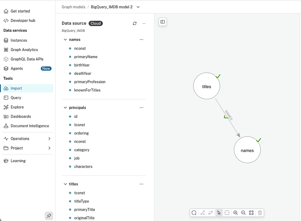
Now it is up to us to change it so that it matches the model above. We change the names of the nodes in line with the Neo4j standard, which is to capitalise the first letter and name them in singular. We also rename names to Person. The relationship we rename to PARTICIPATES_IN. It would have been nice to create different relationships like ACTED_IN, DIRECTED and so on, based on the category, but currently there is no such filter when defining the model. We can, however, refactor the imported model later as we will see in a bit.

We also want to create indexes for the originalTitle and primaryTitle for the Title node, and the primaryName for Person nodes. Finally we need to create the EPISODE_OF relationship from Title to itself, because it was not proposed by the tool. Just drag from the border of the Title node and drop it on itself. Then you fill out the configuration of it like this:

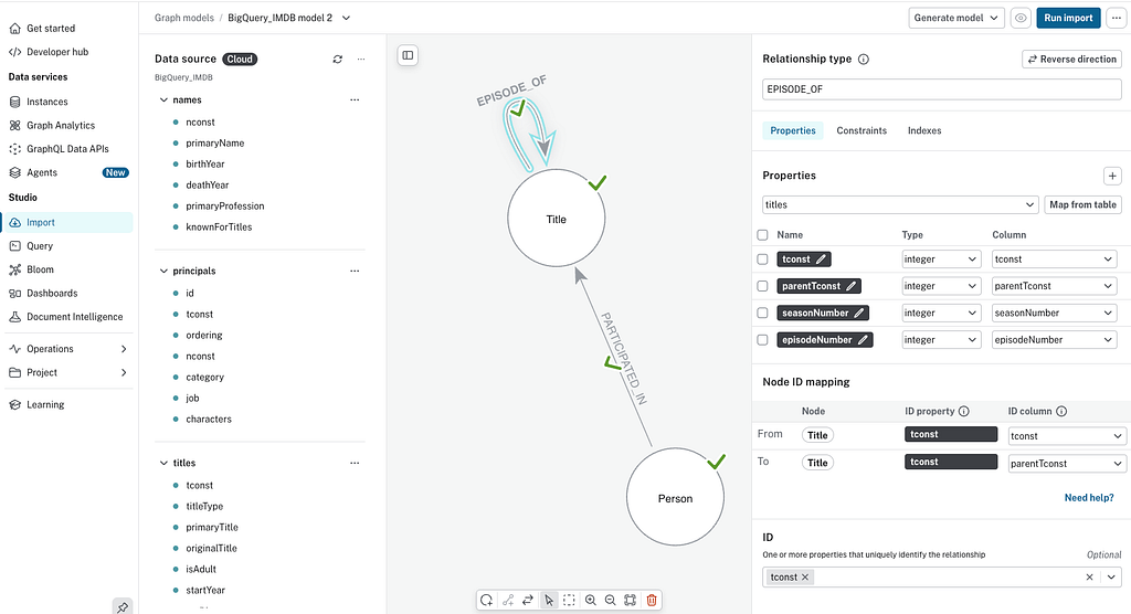
Now we are done with both a data source and a graph model that can be used for both our full ETL and no ETL instance. Since we are in the Import flow right now we’ll start with the ETL version and begin an import job to the BigQuery_IMDB_Import instance we created earlier. Just click the Run import button in the graph modeller, select our BigQuery_IMDB_Import instance and click Run. You will see your import job under the Import jobs tab, and you need to be patient, this will take several hours (depending on the size of the instance you created).

In the meantime we can go ahead and create our no ETL Virtual Graph instance.

Go back to Instances and the Virtual Graphs tab. Click the Create virtual graph button. You will see a dialog which is very similar to the one when we created our native instance, but some fields differ.

I named my instance BigQuery_IMDB_Virtual. The only size option you have is RAM, and the options are 4 GB and 8 GB. Most of the actual query job will be performed by the external system, BigQuery in this case, but depending on the type of query data may have to be collected and post-processed on the Neo4j side, and for those cases more RAM may be needed.

Since we already created our BigQuery data source for the import job we can just select that in the list at the bottom. For BigQuery there is also the possibility to limit the size of data touched by the queries on the BigQuery side. This is a safety since you pay for the amount of data touched by a query when you use BigQuery, and this can become very expensive. The query we will run later will touch less than 4 GB (~2.5 cents), so I will set my limit to 10 GB (6.25 cents with the current price lists of BigQuery).

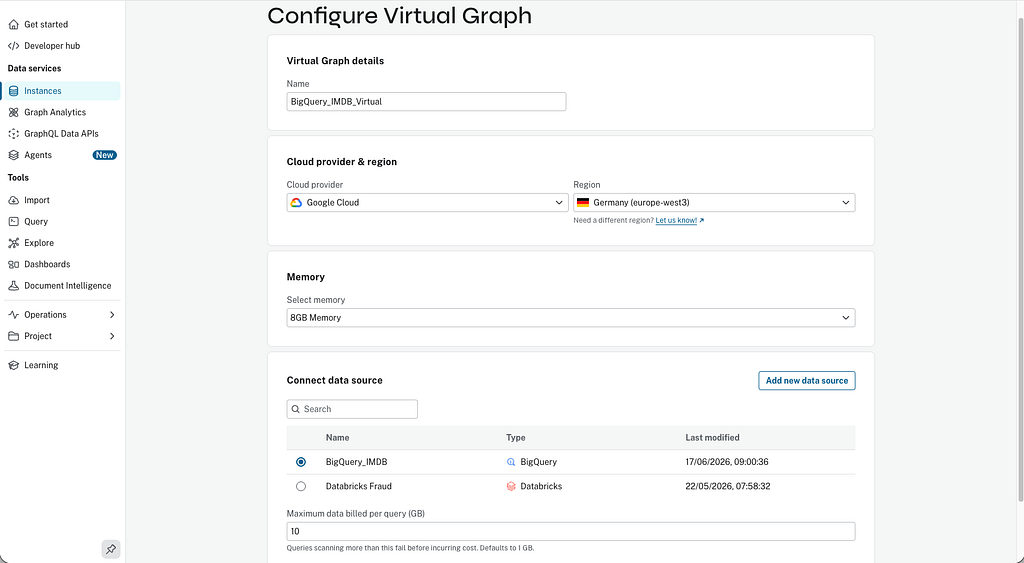
When we are ready we click Next and we now get to choose or create a graph model. Since we will reuse the graph model as well from the import we just click on that in the list of graph models we are presented with, and then click Next again.

Creating the Virtual Graph instance only takes a few minutes, but for this comparison we want to have the other instance ready as well, so we’ll need to wait for the import job to finish. Sit back, have a coffee and read the next chapter while you wait.

Once you have both your instances running you can click the Connect dropdown on the instance and select Query to test the different queries you find below. You can also test the other tools, but we’ll settle with Query here.

Our use case

Our use case will be to look at the Bacon number, or Six degrees of Bacon as it is sometimes called. This is a theory of how interconnected mankind is today. The Bacon number is a metric of how many jumps you have to make through acquaintances to get from yourself to Hollywood actor Kevin Bacon.

My own Bacon number is 2. I know a guy who used to be a sound engineer in Hollywood, and he knows Kevin Bacon. Anyone who knows me has a Bacon number of at most 3.

The theory about the Bacon number states that no-one in the world- no matter how remote you are- have a Bacon number greater than 6.

In Hollywood there is an alternative definition of the Bacon number, which defines how many movies you need to traverse over to get from one actor to Kevin Bacon, by traversing through actors who acted on the same movies.

For my tests here I will look at the Bacon number of Swedish actor Björn Bengtsson, who- in one of his roles- played the Viking warlord Sigefrid in the TV series The Last Kingdom.

Finding the Bacon number

Finding the Bacon number for any actor in our dataset is easily done with a Cypher feature called SHORTEST, which finds the shortest possible path of a pattern expressed, like this:

MATCH p = SHORTEST 1
(:Person {primaryName: "Kevin Bacon", birthYear: 1958})
(()-[:PARTICIPATED_IN {category: "actor"}]
->(:Title {titleType: "movie"})
<-[:PARTICIPATED_IN {category: "actor"}]-())+
(:Person {primaryName: "Björn Bengtsson"})
RETURN size([n IN nodes(p) WHERE n:Title]) AS baconNumber

As you see we specified Björn with just his name and Kevin with birth year as well. This is because there is just one Björn Bengtsson in IMDB, but 7 Kevin Bacons. Just one born in 1958 though.

Running this query on a native Neo4j instance will, as you can see yourself once your import job is completed, only take a fraction of a second, and it will tell us that his Bacon number is 3.

Virtual Graphs does not support SHORTEST and so we cannot run this query on our Virtual instance. But that doesn’t mean we can’t accomplish it. As previously stated, Virtual Graphs supports the different Neo4j tools, and one of those tools is GDS (Graph Data Science), which provides implementations of many specialised graph algorithms. Using GDS Sessions, or Aura Graph Analytics as they are also called, we can run Dijkstra’s algorithm on our dataset to find the shortest path (i.e. the Bacon number).

To use GDS Sessions you start by projecting an in-memory projection of the graph structure (not the full data with properties, just the topology and the IDs — which is why I wanted to make them integers earlier), and for that it will launch a separate compute session (in the projection call we specify the size of the instance and how long we want that to live since there is a cost for having this session running):

MATCH (a:Person)-[:PARTICIPATED_IN {category: 'actor'}]->
      (:Title {titleType: 'movie'})
      <-[:PARTICIPATED_IN {category: 'actor'}]-(b:Person)
WHERE a.nconst < b.nconst
RETURN gds.graph.project(
  'actor-movie-jumps',
  a,
  b,
  {
    sourceNodeLabels: labels(a),
    targetNodeLabels: labels(b),
    relationshipType: 'ACTED_WITH'
  },
  {
    undirectedRelationshipTypes: ['ACTED_WITH'],
    memory: '8GB',
    ttl: duration({hours: 2})
  }
);

We don’t project the movie nodes, since they’re not really needed, we just project the persons and add an ACTED_WITH relationship where they acted on the same movie.

Doing the projection on the Virtual Graph takes just a minute or two, during which the topology has been projected from BigQuery over the Virtual Graph and into the dedicated GDS Session.

For as long as this session is running we can run graph algorithms against the projection. To do the Dijkstra to get the Bacon number of Björn Bengtsson we do:

MATCH (kevin:Person {primaryName: 'Kevin Bacon', birthYear: 1958})
MATCH (bjorn:Person {primaryName: 'Björn Bengtsson'})
CALL gds.shortestPath.dijkstra.stream('actor-movie-jumps', {
  sourceNode: kevin,
  targetNodes: [bjorn]
})
YIELD totalCost
RETURN
  toInteger(totalCost) AS baconNumber

This completes in just a second and gives us the Bacon number of 3, just like the Cypher version on the native graph.

Once we’re done running graph algorithms against our projection we can kill the session. Either we wait the two hours, or we go to Graph Analytics in the Aura console and kill it there.

Cypher: Virtual vs Native

Now we know the Bacon number, but we used different techniques on the native and the virtual graph. To really test the same query on both, let’s rephrase it a bit. Since we know that the Bacon number of Björn is 3 we can instead create a fixed-length query that shows what the 3 hops from Björn to Kevin looks like:

MATCH p = (:Person {primaryName: "Kevin Bacon", birthYear: 1958})-[:PARTICIPATED_IN {category: "actor"}]->
(:Title {titleType: "movie"})
<-[:PARTICIPATED_IN {category: "actor"}]-(:Person)-[:PARTICIPATED_IN {category: "actor"}]->
(:Title {titleType: "movie"})
<-[:PARTICIPATED_IN {category: "actor"}]-(:Person)-[:PARTICIPATED_IN {category: "actor"}]->
(:Title {titleType: "movie"})
<-[:PARTICIPATED_IN {category: "actor"}]-(:Person {primaryName: "Björn Bengtsson"})
RETURN p

(Note that on the native instance we want to run this with the parallel runtime, so we’ll prefix our query with CYPHER runtime = parallel there)

This query will run on both of them, both the native instance and the virtual graph connected to BigQuery. And both of them perform similarly, completing the query in just a few seconds.

This might seem surprising. It is a graph query after all, with a number of jumps in a large, very connected, data set. Why didn’t the native graph outperform the relational one. The first answer is that the query isn’t that complex- the translated SQL query only has 10 JOINs. And the second is that even if BigQuery isn’t a native graph, it is good at using a lot of compute and reading a lot of data efficiently.

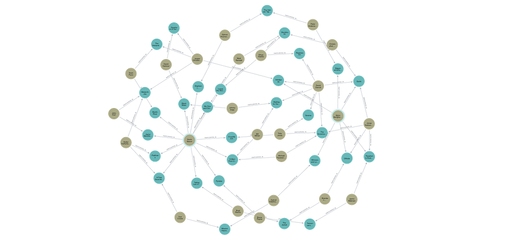
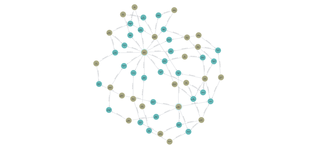
At first sight the two resulting graphs may look different, but that is because of different layouts. On close examination, you will see that they contain the same paths; the same movies, the same actors and the same characters played.

Conclusion

If you have a use case where you haven’t yet chosen where to store the data, then consider the case and choose accordingly. If the data and the use case for accessing the data is tabular in nature, go with a relational data engine, and if it is graph-like go with a graph data engine.

But if you already have a massive amount of data in a data warehouse, like BigQuery, you may want to weigh the benefit of the optimal paradigm with the cost of moving the data. In many cases, as we have seen above, you can get started quickly and solve a lot of the graph algorithms with Virtual Graphs.

It might be that you have real-time requirements, or really complex graph traversals that simply won’t work on a tabular structure, in which case you have to move the data, and for these cases there is the Data Importer in Neo4j. But if that isn’t the case you can at least get started with Virtual Graphs. And if you later want to go full ETL it is really easy to take the step as you already have your data source and graph model defined for the Virtual Graph, and you can just start the importing process using those, while still using the Virtual Graph until it is completed.

In my next blog I will (as already promised) look at a real-world use case that is much more traversal heavy and really benefits from the native graph, but even there you can make it work with Virtual Graphs as long as time isn’t a concern and you can wait for the answer.

Deep-dives

Looking at the generated SQL

If you are using a Virtual Graph instance and you are interested to know what the SQL that it converts your Cypher queries into looks like, you can just prepend your query with EXPLAIN:

EXPLAIN
MATCH p = (:Person {primaryName: "Kevin Bacon", birthYear: 1958})-[:PARTICIPATED_IN {category: "actor"}]->
(:Title {titleType: "movie"})
<-[:PARTICIPATED_IN {category: "actor"}]-(:Person)-[:PARTICIPATED_IN {category: "actor"}]->
(:Title {titleType: "movie"})
<-[:PARTICIPATED_IN {category: "actor"}]-(:Person)-[:PARTICIPATED_IN {category: "actor"}]->
(:Title {titleType: "movie"})
<-[:PARTICIPATED_IN {category: "actor"}]-(:Person {primaryName: "Björn Bengtsson"})
RETURN p

This will, in a standard Neo4j instance, show you the query plan. But in Virtual Graph it will instead show you the SQL that will be sent to the remote data source:

SELECT 
  `unnamed0`.`nconst` AS `unnamed0_nconst`, 
  `unnamed0`.`primaryName` AS `unnamed0_primaryname`, 
  `unnamed0`.`deathYear` AS `unnamed0_deathyear`, 
  `unnamed0`.`primaryProfession` AS `unnamed0_primaryprofession`, 
  `unnamed0`.`birthYear` AS `unnamed0_birthyear`, 
  `unnamed0`.`knownForTitles` AS `unnamed0_knownfortitles`, 
  `unnamed1`.`tconst` AS `unnamed1_tconst`, 
  `unnamed1`.`nconst` AS `unnamed1_nconst`, 
  `unnamed1`.`id` AS `unnamed1_id`, 
  `unnamed1`.`job` AS `unnamed1_job`, 
  `unnamed1`.`category` AS `unnamed1_category`, 
  `unnamed1`.`ordering` AS `unnamed1_ordering`, 
  `unnamed1`.`characters` AS `unnamed1_characters`, 
  `unnamed2`.`tconst` AS `unnamed2_tconst`, 
  `unnamed2`.`originalTitle` AS `unnamed2_originaltitle`, 
  `unnamed2`.`genres` AS `unnamed2_genres`, 
  `unnamed2`.`runtimeMinutes` AS `unnamed2_runtimeminutes`, 
  `unnamed2`.`endYear` AS `unnamed2_endyear`, 
  `unnamed2`.`titleType` AS `unnamed2_titletype`, 
  `unnamed2`.`startYear` AS `unnamed2_startyear`, 
  `unnamed2`.`numVotes` AS `unnamed2_numvotes`, 
  `unnamed2`.`primaryTitle` AS `unnamed2_primarytitle`, 
  `unnamed2`.`averageRating` AS `unnamed2_averagerating`, 
  `unnamed2`.`isAdult` AS `unnamed2_isadult`, 
  `unnamed3`.`tconst` AS `unnamed3_tconst`, 
  `unnamed3`.`nconst` AS `unnamed3_nconst`, 
  `unnamed3`.`id` AS `unnamed3_id`, 
  `unnamed3`.`job` AS `unnamed3_job`, 
  `unnamed3`.`category` AS `unnamed3_category`, 
  `unnamed3`.`ordering` AS `unnamed3_ordering`, 
  `unnamed3`.`characters` AS `unnamed3_characters`, 
  `unnamed4`.`nconst` AS `unnamed4_nconst`, 
  `unnamed4`.`primaryName` AS `unnamed4_primaryname`, 
  `unnamed4`.`deathYear` AS `unnamed4_deathyear`, 
  `unnamed4`.`primaryProfession` AS `unnamed4_primaryprofession`, 
  `unnamed4`.`birthYear` AS `unnamed4_birthyear`, 
  `unnamed4`.`knownForTitles` AS `unnamed4_knownfortitles`, 
  `unnamed5`.`tconst` AS `unnamed5_tconst`, 
  `unnamed5`.`nconst` AS `unnamed5_nconst`, 
  `unnamed5`.`id` AS `unnamed5_id`, 
  `unnamed5`.`job` AS `unnamed5_job`, 
  `unnamed5`.`category` AS `unnamed5_category`, 
  `unnamed5`.`ordering` AS `unnamed5_ordering`, 
  `unnamed5`.`characters` AS `unnamed5_characters`, 
  `unnamed6`.`tconst` AS `unnamed6_tconst`, 
  `unnamed6`.`originalTitle` AS `unnamed6_originaltitle`, 
  `unnamed6`.`genres` AS `unnamed6_genres`, 
  `unnamed6`.`runtimeMinutes` AS `unnamed6_runtimeminutes`, 
  `unnamed6`.`endYear` AS `unnamed6_endyear`, 
  `unnamed6`.`titleType` AS `unnamed6_titletype`, 
  `unnamed6`.`startYear` AS `unnamed6_startyear`, 
  `unnamed6`.`numVotes` AS `unnamed6_numvotes`, 
  `unnamed6`.`primaryTitle` AS `unnamed6_primarytitle`, 
  `unnamed6`.`averageRating` AS `unnamed6_averagerating`, 
  `unnamed6`.`isAdult` AS `unnamed6_isadult`, 
  `unnamed7`.`tconst` AS `unnamed7_tconst`, 
  `unnamed7`.`nconst` AS `unnamed7_nconst`, 
  `unnamed7`.`id` AS `unnamed7_id`, 
  `unnamed7`.`job` AS `unnamed7_job`, 
  `unnamed7`.`category` AS `unnamed7_category`, 
  `unnamed7`.`ordering` AS `unnamed7_ordering`, 
  `unnamed7`.`characters` AS `unnamed7_characters`, 
  `unnamed8`.`nconst` AS `unnamed8_nconst`, 
  `unnamed8`.`primaryName` AS `unnamed8_primaryname`, 
  `unnamed8`.`deathYear` AS `unnamed8_deathyear`, 
  `unnamed8`.`primaryProfession` AS `unnamed8_primaryprofession`, 
  `unnamed8`.`birthYear` AS `unnamed8_birthyear`, 
  `unnamed8`.`knownForTitles` AS `unnamed8_knownfortitles`, 
  `unnamed9`.`tconst` AS `unnamed9_tconst`, 
  `unnamed9`.`nconst` AS `unnamed9_nconst`, 
  `unnamed9`.`id` AS `unnamed9_id`, 
  `unnamed9`.`job` AS `unnamed9_job`, 
  `unnamed9`.`category` AS `unnamed9_category`, 
  `unnamed9`.`ordering` AS `unnamed9_ordering`, 
  `unnamed9`.`characters` AS `unnamed9_characters`, 
  `unnamed10`.`tconst` AS `unnamed10_tconst`, 
  `unnamed10`.`originalTitle` AS `unnamed10_originaltitle`, 
  `unnamed10`.`genres` AS `unnamed10_genres`, 
  `unnamed10`.`runtimeMinutes` AS `unnamed10_runtimeminutes`, 
  `unnamed10`.`endYear` AS `unnamed10_endyear`, 
  `unnamed10`.`titleType` AS `unnamed10_titletype`, 
  `unnamed10`.`startYear` AS `unnamed10_startyear`, 
  `unnamed10`.`numVotes` AS `unnamed10_numvotes`, 
  `unnamed10`.`primaryTitle` AS `unnamed10_primarytitle`, 
  `unnamed10`.`averageRating` AS `unnamed10_averagerating`, 
  `unnamed10`.`isAdult` AS `unnamed10_isadult`, 
  `unnamed11`.`tconst` AS `unnamed11_tconst`, 
  `unnamed11`.`nconst` AS `unnamed11_nconst`, 
  `unnamed11`.`id` AS `unnamed11_id`, 
  `unnamed11`.`job` AS `unnamed11_job`, 
  `unnamed11`.`category` AS `unnamed11_category`, 
  `unnamed11`.`ordering` AS `unnamed11_ordering`, 
  `unnamed11`.`characters` AS `unnamed11_characters`, 
  `unnamed12`.`nconst` AS `unnamed12_nconst`, 
  `unnamed12`.`primaryName` AS `unnamed12_primaryname`, 
  `unnamed12`.`deathYear` AS `unnamed12_deathyear`, 
  `unnamed12`.`primaryProfession` AS `unnamed12_primaryprofession`, 
  `unnamed12`.`birthYear` AS `unnamed12_birthyear`, 
  `unnamed12`.`knownForTitles` AS `unnamed12_knownfortitles` 
FROM 
  `[PROJECT]`.`imdb`.`names` AS `unnamed0` 
  JOIN `[PROJECT]`.`imdb`.`principals` AS `unnamed1` ON `unnamed1`.`nconst` = `unnamed0`.`nconst` 
  JOIN `[PROJECT]`.`imdb`.`titles` AS `unnamed2` ON `unnamed2`.`tconst` = `unnamed1`.`tconst` 
  JOIN `[PROJECT]`.`imdb`.`principals` AS `unnamed3` ON `unnamed3`.`tconst` = `unnamed2`.`tconst` 
  JOIN `[PROJECT]`.`imdb`.`names` AS `unnamed4` ON `unnamed4`.`nconst` = `unnamed3`.`nconst` 
  JOIN `[PROJECT]`.`imdb`.`principals` AS `unnamed5` ON `unnamed5`.`nconst` = `unnamed4`.`nconst` 
  JOIN `[PROJECT]`.`imdb`.`titles` AS `unnamed6` ON `unnamed6`.`tconst` = `unnamed5`.`tconst` 
  JOIN `[PROJECT]`.`imdb`.`principals` AS `unnamed7` ON `unnamed7`.`tconst` = `unnamed6`.`tconst` 
  JOIN `[PROJECT]`.`imdb`.`names` AS `unnamed8` ON `unnamed8`.`nconst` = `unnamed7`.`nconst` 
  JOIN `[PROJECT]`.`imdb`.`principals` AS `unnamed9` ON `unnamed9`.`nconst` = `unnamed8`.`nconst` 
  JOIN `[PROJECT]`.`imdb`.`titles` AS `unnamed10` ON `unnamed10`.`tconst` = `unnamed9`.`tconst` 
  JOIN `[PROJECT]`.`imdb`.`principals` AS `unnamed11` ON `unnamed11`.`tconst` = `unnamed10`.`tconst` 
  JOIN `[PROJECT]`.`imdb`.`names` AS `unnamed12` ON `unnamed12`.`nconst` = `unnamed11`.`nconst` 
WHERE 
  (`unnamed0`.`primaryName` = ? /*autostring0*/) 
  AND (`unnamed0`.`birthYear` = ? /*autoint1*/) 
  AND (`unnamed1`.`category` = ? /*autostring2*/) 
  AND (`unnamed2`.`titleType` = ? /*autostring3*/) 
  AND (`unnamed3`.`category` = ? /*autostring4*/) 
  AND (`unnamed5`.`category` = ? /*autostring5*/) 
  AND (`unnamed6`.`titleType` = ? /*autostring6*/) 
  AND (`unnamed7`.`category` = ? /*autostring7*/) 
  AND (`unnamed9`.`category` = ? /*autostring8*/) 
  AND (`unnamed10`.`titleType` = ? /*autostring9*/) 
  AND (`unnamed11`.`category` = ? /*autostring10*/) 
  AND (`unnamed12`.`primaryName` = ? /*autostring11*/) 
  AND (NOT ((`unnamed11`.`tconst` = `unnamed9`.`tconst`) AND (`unnamed11`.`nconst` = `unnamed9`.`nconst`) AND (`unnamed11`.`id` = `unnamed9`.`id`))) 
  AND (NOT ((`unnamed11`.`tconst` = `unnamed7`.`tconst`) AND (`unnamed11`.`nconst` = `unnamed7`.`nconst`) AND (`unnamed11`.`id` = `unnamed7`.`id`))) 
  AND (NOT ((`unnamed11`.`tconst` = `unnamed5`.`tconst`) AND (`unnamed11`.`nconst` = `unnamed5`.`nconst`) AND (`unnamed11`.`id` = `unnamed5`.`id`))) 
  AND (NOT ((`unnamed11`.`tconst` = `unnamed3`.`tconst`) AND (`unnamed11`.`nconst` = `unnamed3`.`nconst`) AND (`unnamed11`.`id` = `unnamed3`.`id`))) 
  AND (NOT ((`unnamed11`.`tconst` = `unnamed1`.`tconst`) AND (`unnamed11`.`nconst` = `unnamed1`.`nconst`) AND (`unnamed11`.`id` = `unnamed1`.`id`))) 
  AND (NOT ((`unnamed9`.`tconst` = `unnamed7`.`tconst`) AND (`unnamed9`.`nconst` = `unnamed7`.`nconst`) AND (`unnamed9`.`id` = `unnamed7`.`id`))) 
  AND (NOT ((`unnamed9`.`tconst` = `unnamed5`.`tconst`) AND (`unnamed9`.`nconst` = `unnamed5`.`nconst`) AND (`unnamed9`.`id` = `unnamed5`.`id`))) 
  AND (NOT ((`unnamed9`.`tconst` = `unnamed3`.`tconst`) AND (`unnamed9`.`nconst` = `unnamed3`.`nconst`) AND (`unnamed9`.`id` = `unnamed3`.`id`))) 
  AND (NOT ((`unnamed9`.`tconst` = `unnamed1`.`tconst`) AND (`unnamed9`.`nconst` = `unnamed1`.`nconst`) AND (`unnamed9`.`id` = `unnamed1`.`id`))) 
  AND (NOT ((`unnamed7`.`tconst` = `unnamed5`.`tconst`) AND (`unnamed7`.`nconst` = `unnamed5`.`nconst`) AND (`unnamed7`.`id` = `unnamed5`.`id`))) 
  AND (NOT ((`unnamed7`.`tconst` = `unnamed3`.`tconst`) AND (`unnamed7`.`nconst` = `unnamed3`.`nconst`) AND (`unnamed7`.`id` = `unnamed3`.`id`))) 
  AND (NOT ((`unnamed7`.`tconst` = `unnamed1`.`tconst`) AND (`unnamed7`.`nconst` = `unnamed1`.`nconst`) AND (`unnamed7`.`id` = `unnamed1`.`id`))) 
  AND (NOT ((`unnamed5`.`tconst` = `unnamed3`.`tconst`) AND (`unnamed5`.`nconst` = `unnamed3`.`nconst`) AND (`unnamed5`.`id` = `unnamed3`.`id`))) 
  AND (NOT ((`unnamed5`.`tconst` = `unnamed1`.`tconst`) AND (`unnamed5`.`nconst` = `unnamed1`.`nconst`) AND (`unnamed5`.`id` = `unnamed1`.`id`))) 
  AND (NOT ((`unnamed3`.`tconst` = `unnamed1`.`tconst`) AND (`unnamed3`.`nconst` = `unnamed1`.`nconst`) AND (`unnamed3`.`id` = `unnamed1`.`id`)));

Optimising the graph

In the earlier chapter when we compared native graphs and virtual graphs, they both took a couple of seconds on both variants. Part of this is because we had a string property predicate on every node and relationship in our pattern. So as it traversed it had to do string compares on every jump evaluated. We can solve that by modelling our graph with dedicated node labels and relationship types. We can refactor our native graph like this:

MATCH (a)-[p:PARTICIPATED_IN {category: "actor"}]->(b)
CALL(a,b,p) {
    MERGE (a)-[r:ACTED_IN]->(b)
    ON CREATE SET r = properties(p)
} IN TRANSACTIONS OF 100000 ROWS;

MATCH (m:Title&!Movie {titleType: "movie"})
CALL(m) {
    SET m:Movie
} IN TRANSACTIONS OF 100000 ROWS;

Now we have added an ACTED_IN relationship for all PARTICIPATED_IN that had category “actor”, and a Movie label to all Title nodes where titleType was “movie”. With that we can rewrite our query without predicates on anything but the start and end node:

CYPHER runtime=parallel
MATCH p = (:Person {primaryName: "Kevin Bacon", birthYear: 1958})-[:ACTED_IN]->
(:Movie)<-[:ACTED_IN]-(:Person)-[:ACTED_IN]->
(:Movie)<-[:ACTED_IN]-(:Person)-[:ACTED_IN]->
(:Movie)<-[:ACTED_IN]-(:Person {primaryName: "Björn Bengtsson"})
RETURN p

This makes the query run 2–4 times faster on the native graph. But what about the Virtual Graph? Well, we can’t refactor it from within the virtual graph. But we can do something similar in BigQuery before creating the Virtual Graph (and in that case also doing that before importing the data, and thus not needing the refactoring above). Just run this in BigQuery:

CREATE OR REPLACE VIEW imdb.v_movies AS SELECT * FROM imdb.titles WHERE titleType = 'movie';
CREATE OR REPLACE VIEW imdb.v_actors AS SELECT * FROM imdb.principals WHERE category = 'actor';

Now we can create a new graph model in Neo4j based on these views and start a new Virtual Graph instance based on the same data source, but this new graph model.

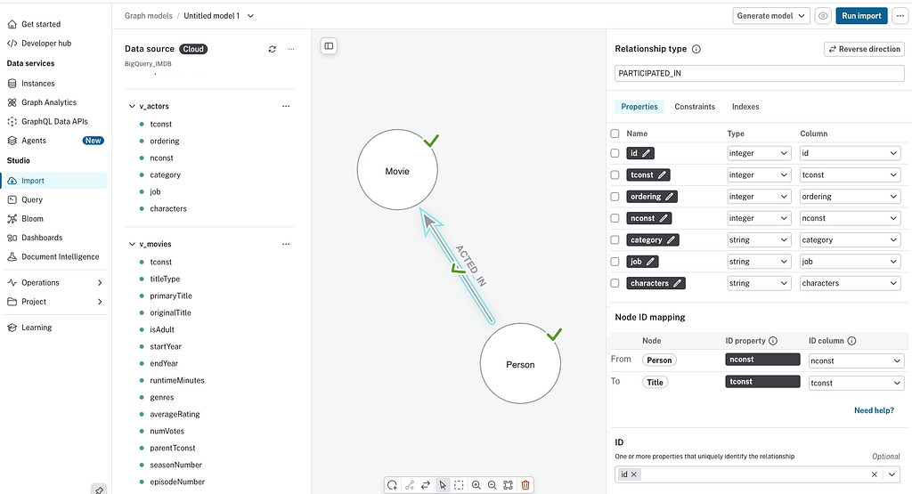
And now we can run this query with the Virtual Graph as well:

MATCH p = (:Person {primaryName: "Kevin Bacon", birthYear: 1958})-[:ACTED_IN]->
(:Movie)<-[:ACTED_IN]-(:Person)-[:ACTED_IN]->
(:Movie)<-[:ACTED_IN]-(:Person)-[:ACTED_IN]->
(:Movie)<-[:ACTED_IN]-(:Person {primaryName: "Björn Bengtsson"})
RETURN p

BigQuery Graph

There is also a way to run GQL (~Cypher) queries directly within BigQuery. If you click the dots next to your dataset you can select Create Graph. This allows you to define a graph model, similar to what we did for our Virtual Graph, and then run GQL queries against that.

BigQuery has good support for expressing graph patterns, but you cannot return graph elements such as paths, nodes or relationships. So we cannot run the query we used earlier. But instead of returning the path p, we can return the number of 3-movie paths found.

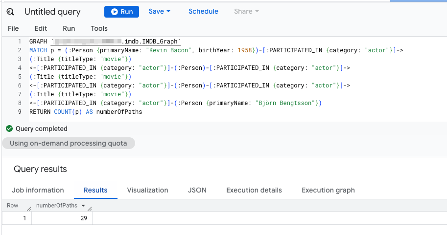
It gives the expressiveness of Cypher, but without the graph visualisations. It is sort of like the SAAB, looking like a SAAB, but with the comfortable seats from the Porsche.

Still it gives you a way to test writing Cypher/GQL queries before launching either a Virtual Graph or importing your data into a native graph.

---

Deep Dive: Neo4j Virtual Graph on BigQuery was originally published in Neo4j Developer Blog on Medium, where people are continuing the conversation by highlighting and responding to this story.