Data exploration with the Neo4j Runway Python library

Senior AI Solutions Architect, Neo4j
13 min read

Explore and ingest your relational data into a Neo4j graph in minutes

Introduction
Neo4j Runway is a Python library I developed with the help of Jason Booth and Daniel Bukowski at Neo4j. It provides tools that abstract communication with OpenAI to run discovery on your data and generate a data model, and tools to generate ingestion code and load your data into a Neo4j instance. The goal is to simplify the user experience of understanding how their relational data can fit into a graph data model and get them exploring quickly.
The information in this article pertains to Neo4j Runway v0.2.2
Key features
- Data discovery: Harness OpenAI LLMs to provide valuable insights from your data.
- Graph data modeling: Use OpenAI and the Instructor Python library to create valid graph data models.
- Code generation: Generate ingestion code for your preferred method of loading data.
- Data ingestion: Load your data using Runway’s built-in implementation of pyingest — a Neo4j Python ingestion tool.
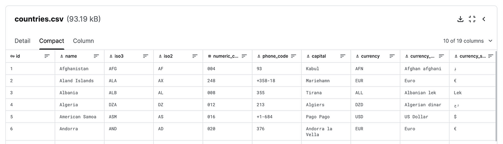
We’ll walk through these key features by exploring a CSV file containing data on countries. The data can be found in the repo link or on Kaggle.
The notebook we’ll use as a guide is in this repo of examples using the Neo4j Runway library: countries.ipynb.
neo4j-runway-examples/countries.ipynb at main · a-s-g93/neo4j-runway-examples
Requirements
Runway uses Graphviz to visualize data models. To use this feature, download Graphviz. This install is necessary to run the Graphviz Python package.
You’ll need a Neo4j instance to use Runway fully. Start a free cloud-hosted Aura instance or download the Neo4j Desktop app.
Neo4j Runway requires an OpenAI API key to use the discovery and data model generation modules. The ingestion code generation and data ingestion modules do not require access to an LLM.
To install, simply run this pip command:
pip install neo4j-runway
Runway is still in beta. Feel free to provide feedback and report any bugs.
Discovery
Discovery is a significant step in migrating data into a graph. It makes us pause to understand the relationships among features, which features may not be necessary, nodes that may not be supported due to missing data, and much more. We can expedite this process by asking an LLM to help us discover these insights.
The Discovery module generates rich context for the data modeling stage. You may pass it user input as a Python dictionary or a UserInput object. This input contains a general description of the CSV data and descriptions of each column you’d like to use in your graph data model:
USER_GENERATED_INPUT = {
'general_description': 'This is data on different countries.',
'id': 'unique id for a country.',
'name': 'the country name.',
'phone_code': 'country area code.',
'capital': 'the capital of the country.',
'currency_name': "name of the country's currency.",
'region': 'primary region of the country.',
'subregion': 'subregion location of the country.',
'timezones': 'timezones contained within the country borders.',
'latitude': 'the latitude coordinate of the country center.',
'longitude': 'the longitude coordinate of the country center.'
}
Or:
USER_GENERATED_INPUT = UserInput(
general_description='This is data on different countries.',
column_descriptions={
'id': 'unique id for a country.',
'name': 'the country name.',
'phone_code': 'country area code.',
'capital': 'the capital of the country.',
'currency_name': "name of the country's currency.",
'region': 'primary region of the country.',
'subregion': 'subregion location of the country.',
'timezones': 'timezones contained within the country borders.',
'latitude': 'the latitude coordinate of the country center.',
'longitude': 'the longitude coordinate of the country center.'
}
)
The user input discussed above is optional, but can lead to better results. If no column descriptions dictionary is provided, all columns will be considered for use in the data model by default.
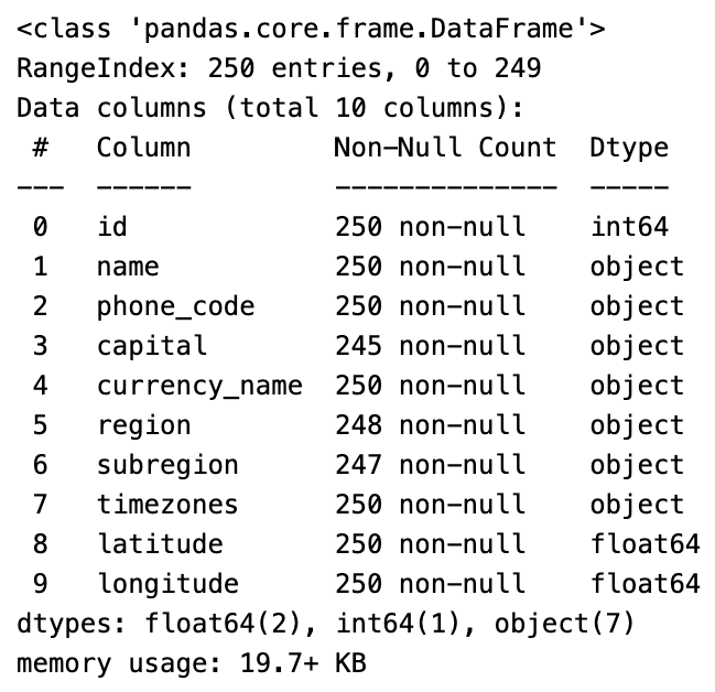
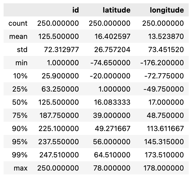
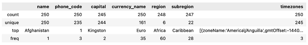
The Discovery module then uses pandas to create general, numeric, and categorical data descriptions. This is then passed with the provided user input in a prompt to an OpenAI LLM to generate additional findings. We can see the generated pandas descriptions for our country data below.
Let’s get started by importing the modules we’ll use and read in our data using the pandas read_csv method:
import os

import pandas as pd
from dotenv import load_dotenv

from neo4j_runway import (Discovery, GraphDataModeler,
                          IngestionGenerator, LLM, PyIngest)
from neo4j_runway.utils import test_database_connection

load_dotenv()

data = pd.read_csv("data/csv/countries.csv")
We then initialize our LLM. By default, we use GPT-4o and define our OpenAI API key in an environment variable. You may also pass your API key and desired LLM model directly to the LLM constructor:
llm = LLM(model="gpt-4o-2024-05-13", open_ai_key="sk-...")
Now we can run discovery on our data:
disc = Discovery(llm=llm, user_input=USER_GENERATED_INPUT, data=data)
disc.run()
The Markdown discovery generated by the LLM:
Based on the provided summary and description of the data, here is a preliminary analysis:

### Overall Details:
1. **Data Completeness**:
   - The dataset contains 250 entries (countries) and 10 features.
   - Most features are complete, but there are some missing values:
     - `capital`: 5 missing values.
     - `region`: 2 missing values.
     - `subregion`: 3 missing values.

2. **Data Types**:
   - The dataset includes a mix of data types:
     - Numerical: `id`, `latitude`, `longitude`.
     - Categorical: `name`, `phone_code`, `capital`, `currency_name`, `region`, `subregion`, `timezones`.

3. **Unique Values**:
   - `name`: All 250 entries are unique.
   - `phone_code`: 235 unique values, with the most common code appearing 3 times.
   - `capital`: 244 unique values, with one capital appearing twice.
   - `currency_name`: 161 unique values, with "Euro" being the most common (35 occurrences).
   - `region`: 6 unique values, with "Africa" being the most common (60 occurrences).
   - `subregion`: 22 unique values, with "Caribbean" being the most common (28 occurrences).
   - `timezones`: 245 unique values, with the most common timezone appearing 3 times.

### Important Features:
1. **Geographical Coordinates**:
   - `latitude` and `longitude` provide the geographical center of each country. These features are crucial for spatial analysis and mapping.

2. **Country Identification**:
   - `id` and `name` uniquely identify each country. These are essential for referencing and linking data.

3. **Administrative and Political Information**:
   - `capital`: Provides the capital city, which is often a key administrative and political center.
   - `region` and `subregion`: These features categorize countries into broader geographical and political groupings, useful for regional analysis.

4. **Economic Information**:
   - `currency_name`: Indicates the currency used, which can be important for economic and financial analysis.

5. **Communication**:
   - `phone_code`: Provides the country’s area code, useful for telecommunications and international dialing.

6. **Time Zones**:
   - `timezones`: Lists the time zones within each country, which is important for understanding temporal differences and scheduling across regions.

### Summary:
- The dataset is relatively complete with only a few missing values.
- It contains a mix of numerical and categorical data, with unique identifiers for each country.
- Key features include geographical coordinates, administrative information (capital, region, subregion), economic data (currency), and communication details (phone code, timezones).
- The data is well-suited for geographical, political, and economic analysis, and can be used to explore relationships between countries based on these features.

This preliminary analysis provides a foundation for further exploration and potential modeling, including the creation of a graph data model.
Graph data modeling
The GraphDataModeler will take the discovery information and attempt to create a valid graph data model. Here, we use the same LLM used in the discovery process — however, this isn’t necessary. I found that GPT-3.5 was sufficient for the discovery process, but a GPT-4 variant was usually required to receive a usable data model.
The generated data model will also have Neo4j naming conventions applied automatically, so labels are PascalCase, relationships are SCREAMING_SNAKE_CASE, and properties are camelCase.
gdm = GraphDataModeler(llm=llm, discovery=disc)
gdm.create_initial_model()
If we have Graphviz installed, we can take a look at our model:
gdm.current_model.visualize()
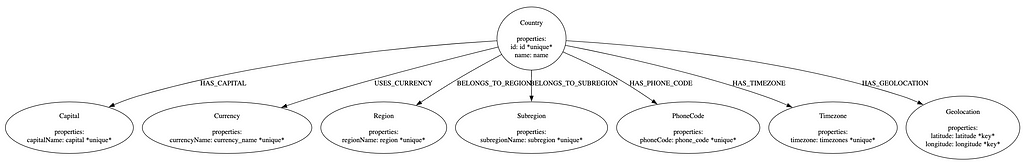
Runway allows us to iterate on our model by providing feedback. Let’s make some corrections to our model and view the results:
gdm.iterate_model(user_corrections="""
Make Region node have a HAS_SUBREGION relationship with Subregion node.
Remove The relationship between Country and Region.
Both the latitude and longitude properties on Geolocation should remain node keys.
""")
gdm.current_model.visualize()
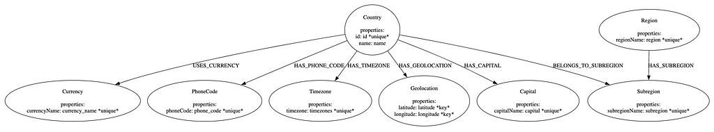
Notice that each node has either a unique property or node keys. Sometimes the LLM may not identify these on the first data model, so it is recommended to iterate on the data model at least once — even if no corrections are provided. We won’t be able to ingest our data without this information.
By default iteration prompt will ask the LLM to consider new nodes and properties from the CSV.
We can continue to iterate on the model in Runway or we can export the model with the to_arrows() method and manually modify it in Neo4j’s arrows.app web application. Arrows.app integration is detailed in this article. For now let’s continue with the current data model.
Leveraging LLMs
The Discovery and Data Modeling modules rely on LLMs to generate meaningful output. Discovery is relatively easy to orchestrate, but data modeling is more difficult.
We use the Instructor Python library to control the LLM output with a Pydantic model. This works by guiding the LLM to output JSON that matches the graph data model and retrying the LLM call if the output JSON doesn’t accurately map to the Pydantic model representation. Each retry will include the Pydantic error messages so that the LLM can correct itself. This Instructor-based validation stage may occur up to three times.
Welcome To Instructor – Instructor
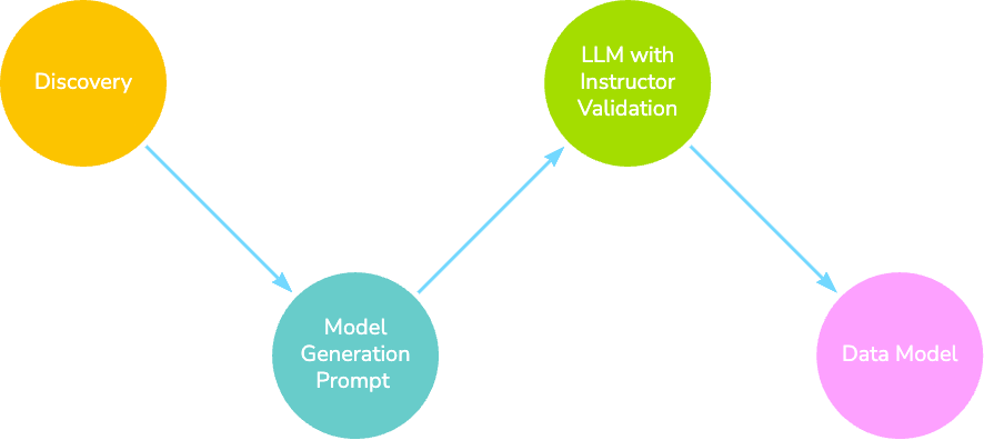
To generate our initial data model, we simply pass the information gathered from the Discovery class into a prompt containing some rules and the generic data model format.
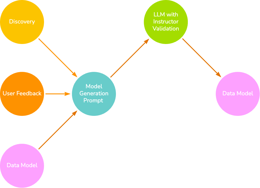
Once we have our first data model, we can provide feedback to improve it. This involves passing the Discovery information along with the previous model and any feedback.
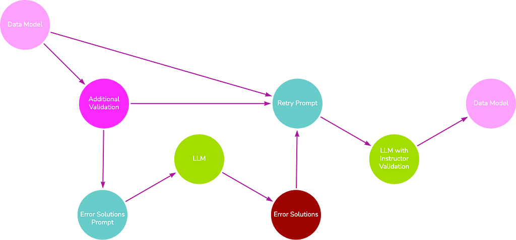
Once a model passes the initial Instructor validation, we enforce additional validation, such as relationship source and target existence, unique property duplication, and node/relationship property name to CSV column name mapping.
If these fail, we perform chain-of-thought prompting by first asking the LLM how it will solve the present errors, then feeding that response back into the LLM to receive a new valid data model, we hope. By default, this process may occur up to three times.
Model generation can only be attempted a finite number of times before the process terminates and either an error (the LLM fails to create a data model that adheres to the Pydantic model) or the unfinished model is returned (the additional validation stage fails and reached the max number of retries). These outcomes are less likely if:
- You are using an LLM ≥ GPT-4.
- Meaningful data and feature descriptions are provided in the user input.
- Your CSV data is healthy and consistent.
Code generation
Runway supports two code generation options: LOAD CSV and PyIngest YAML configuration. Both of these methods generate the necessary Cypher code to create constraints and load your CSV data, but the format is slightly different to accommodate preferred ingestion methods. In this example, we generate a PyIngest config YAML to use with Runway’s built-in modified version of PyIngest. We can pass the current data model with the current_model property of the GraphDataModeler class. We also need to include the CSV directory and CSV name. Optionally, we can provide connection credentials directly in the class constructor or we can manually enter these fields in the YAML file once generated.
The CSV name argument will overwrite any csv_name properties on nodes and relationships. This argument should only be provided if data is from a single CSV. Currently, data model generation via LLM only supports single CSV data, but imported data models from arrows.app may have multiple CSVs.
gen = IngestionGenerator(data_model=gdm.current_model,
username="neo4j", password="password",
uri="bolt://localhost:7687", database="neo4j",
csv_dir="data/csv/", csv_name="countries.csv")

pyingest_yaml = gen.generate_pyingest_yaml_string()
To save the YAML file, we can run the following instead:
gen.generate_pyingest_yaml_file(file_name="countries")
Ingestion
Neo4j Runway provides a built-in ingestion function via a modified PyIngest file. This version takes the configuration YAML generated above and an optional pandas DataFrame as input. It then loads the data into a graph according to the credentials provided in the YAML. The original PyIngest is much more flexible in terms of file format and storage location and is 100-percent compatible with the configuration file generated by Runway. So if you need another option for loading your data, feel free to use that or the LOAD CSV method instead.
Let’s confirm our database connection by using the test_database_connection function:
test_database_connection(credentials={"username": os.environ.get("NEO4J_USERNAME"), "password": os.environ.get("NEO4J_PASSWORD"), "uri": os.environ.get("NEO4J_URI")})
If the connection is successful, we should receive the following response:
{'valid': True, 'message': 'Connection and Auth Verified!'}
To load our data, we simply run:
PyIngest(yaml_string=pyingest_yaml, dataframe=data)
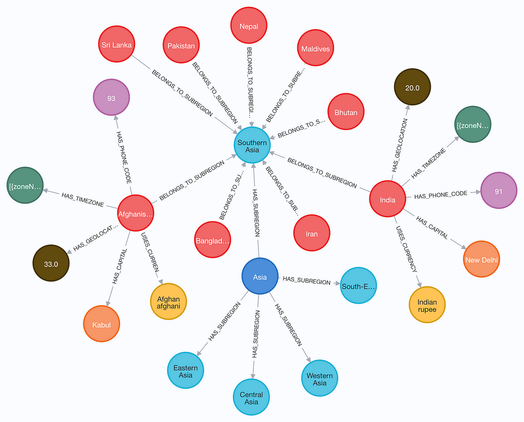
And finally, here’s a snapshot of the generated graph.
Conclusion
Neo4j Runway is an easy-to-use tool to explore your data as a graph. It guides you through the process from data discovery to loading your data into a database. Although all four primary modules are built to complement each other, it is not necessary to use them all. Data modeling is more successful when provided with a Discovery object, but it is not required to function. It is also possible to design a data model in arrows.app and import it into Runway for code generation and ingestion. The arrows.app integration is detailed in this article.
Please remember that Runway is still in beta. Feel free to provide feedback and report any bugs.
Data Exploration With the Neo4j Runway Python Library was originally published in Neo4j Developer Blog on Medium, where people are continuing the conversation by highlighting and responding to this story.
Share Article


Explore
Related Articles

Neo4j Named “One to Watch” in Snowflake’s 2026 Modern Marketing Data Stack Report