Speed up your queries with Neo4j’s new parallel runtime


16 min read

The new Parallel Cypher Runtime is a fantastic alternative for executing graph-global read queries, but you should know when to use it.

Most users of Neo4j will probably not have meddled too much with Cypher runtimes (some may not even know what a runtime is). Nor should they — pipelined runtime (the default runtime for Enterprise Edition) is designed to provide the best query performance for the most common use cases.
However, there are cases in which pipelined runtime is not ideal, like running analytical queries that process a large part of your graph. Luckily, the new Cypher runtime, parallel runtime (introduced in Neo4j 5.13), excels in many of those cases by drastically improving the speed of particular types of queries.
In this blog, we’ll briefly explain what a query runtime is and then go a little deeper into some of the situations where the new parallel runtime shines.
For readers with less time on their hands, this is the TL;DR — parallel runtime is a fantastic alternative for taking advantage of the available CPUs to execute graph-global read queries, but it should not be considered a comprehensive replacement for pipelined runtime.
Data model
In this blog, we will be using data from a full Stack Overflow dump, containing the following nodes (53M) and relationships (120M):
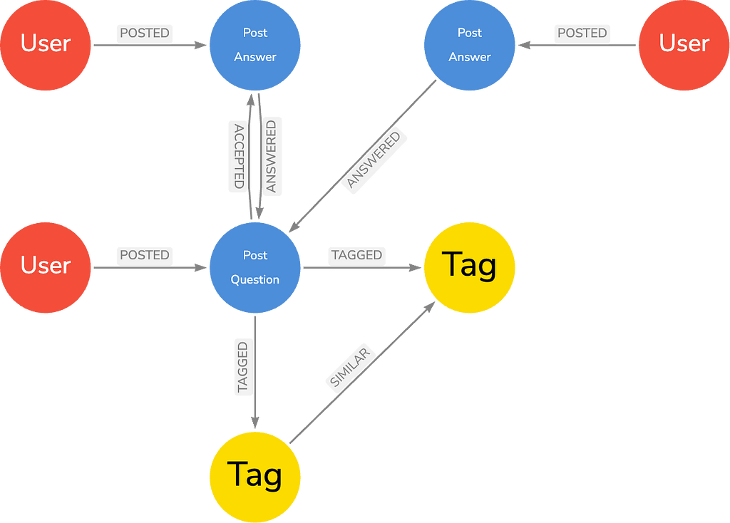
As can be seen from a glimpse of the data model, the node labels and relationship types present in the graph can be used to look for patterns in user behavior on Stack Overflow, which is exactly what we will be doing in just a little bit…
Runtimes and the life of a Cypher query
Before we look at the awesome potential of parallel runtime in particular, we first need to answer a more basic set of questions:
What is a runtime? And what role does it play in a Cypher query?
MATCH (t:Tag {name:'neo4j'})<-[:TAGGED]-(q:Question)
MATCH (q)-[:ACCEPTED]->(a:Answer)<-[:POSTED]-(u:User)
WITH u, count(*) as freq
ORDER BY freq DESC LIMIT 5
RETURN u.name, freq
A Cypher query begins life as a string containing information about what particular pattern in the graph to match. That string is processed by the query parser and turned into an internal representation (Abstract Syntax Tree — AST), which is checked and cleaned up. That AST is received by a query optimizer, also known as the planner, which creates a plan for how the query should be executed.
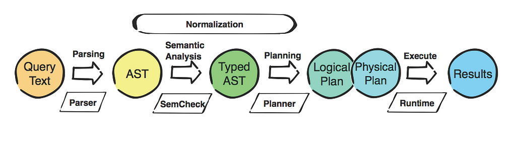
This plan is composed of different operators — specialized execution modules that perform a specific transformation task on the data — which tell you how a query will be evaluated to obtain the desired result.
Once the query plan has been produced, the query runtime takes over to actually execute the plan produced by the planner against the database as quickly and efficiently as possible.
Pipelines and threads
To understand the purpose of parallel runtime, it will be helpful to consider briefly some of the ways it is similar and different to the pipelined runtime, which is — and will continue to be — the default runtime for Neo4j Enterprise Edition and all tiers of Aura.
Fundamentally, the pipelined and parallel runtimes share the same architecture in that they are both pipelined. This means that rather than executing queries one row at a time (as in slotted runtime — the default runtime in Neo4j Community Edition), operators are grouped into pipelines that work on a batch of rows at a time.
To show pipelines in action, consider a query (run with pipelined runtime) that asks for the trends in which days of a month in a particular year that Stack Overflow sees the most activity:
CALL {
  MATCH (p:Post)
  WITH
    CASE
      WHEN p.updatedAt IS NULL THEN [p.createdAt]
      ELSE [p.createdAt, p.updatedAt]
    END AS activityDates
  UNWIND activityDates AS activityDate
  RETURN activityDate
  UNION ALL
  MATCH (u:User)
  UNWIND [u.createdAt, u.accessedAt] AS activityDate
  RETURN activityDate
}
RETURN activityDate.year AS year,
       activityDate.month AS month,
       count(*) AS activity
ORDER BY activity DESC, year, month
LIMIT 10
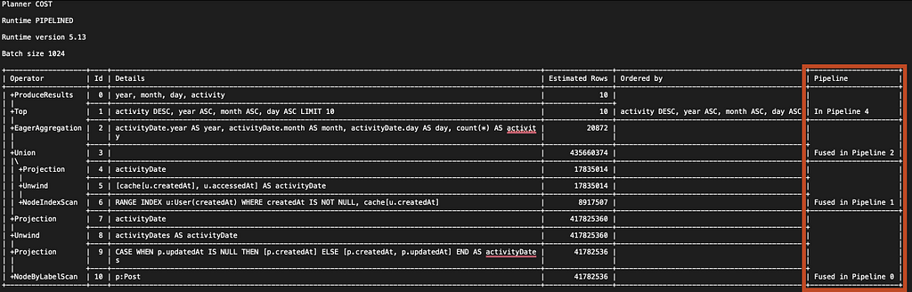
It generates the following execution plan, where, in the rightmost column, we can see that it has been divided into 4 separate pipelines, all containing 2 or more operators.
Both pipelined and parallel runtimes execute rows in batches. However, while pipelined runtime can only execute one batch at a time, parallel runtime executes multiple batches simultaneously.
This is possible because, while pipelined runtime is considered a single-threaded runtime, where each batch is processed by a single thread assigned to one CPU core, parallel runtime is a multi-threaded runtime, which allows for multiple batches to be processed simultaneously by the available CPUs.
In essence, this is why parallel runtime brings a new ability for Neo4j users to take advantage of the number of available CPUs to significantly speed up the execution of their queries.
But enough theory. Let’s run some actual queries with parallel runtime!
Faster graph-global queries
The ability of parallel runtime to utilize many CPUs means that it is ideal for graph-global queries. These are queries that do not specify any particular node as a starting point and proceed to traverse a large part of the graph to uncover complex patterns.
Let’s look at how a few graph-global queries perform on the two different runtimes when run on a machine with 16 cores.
We start with the previous query (which qualifies as a graph-global query). When run with pipelined runtime, we see that it takes 53,790 milliseconds, or just under a minute, to complete.

Now, we run it with parallel runtime instead. To do this, prepend the query with CYPHER runtime=parallel:
CYPHER runtime=parallel
CALL {
  MATCH (p:Post)
  WITH
    CASE
      WHEN p.updatedAt IS NULL THEN [p.createdAt]
      ELSE [p.createdAt, p.updatedAt]
    END AS activityDates
  UNWIND activityDates AS activityDate
  RETURN activityDate
  UNION ALL
  MATCH (u:User)
  UNWIND [u.createdAt, u.accessedAt] AS activityDate
  RETURN activityDate
}
RETURN activityDate.year AS year,
       activityDate.month AS month,
       count(*) AS activity
ORDER BY activity DESC, year, month
LIMIT 10
Et Voila! The query time is down to 9757 milliseconds, almost a sixth of the time it took to complete with pipelined runtime!

The fundamental reason for parallel runtime being so much faster in this case is that it can process many pipeline tasks simultaneously (in parallel).
Parallelism is achieved along two dimensions:
- “vertically” (tasks of different pipelines can execute in parallel), and
- “horizontally” (multiple tasks of the same pipeline can execute in parallel).
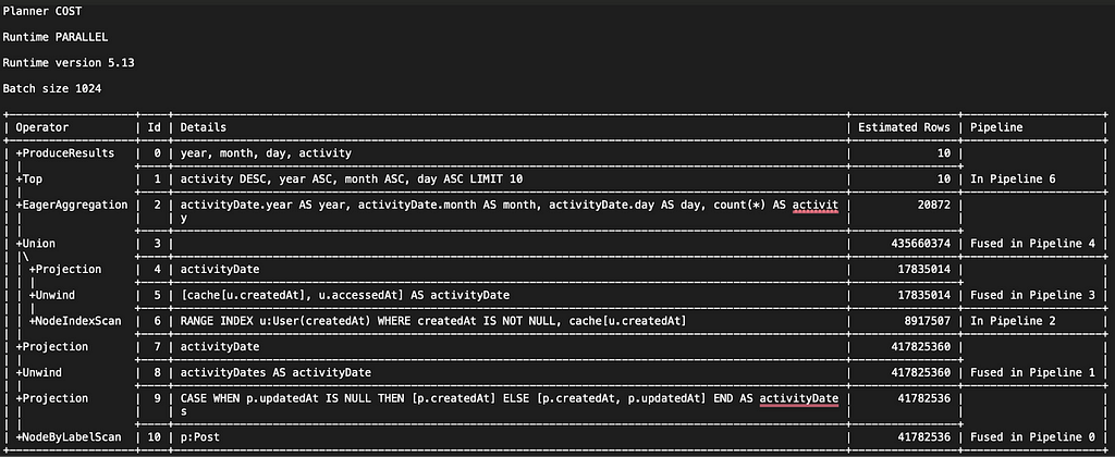
One detail that allows parallel runtime to maximize “vertical” parallelism opportunities is that it splits plans into more, smaller pipelines, enabling the runtime to work on more pipelines simultaneously. And, sticking with the same example, we see that the execution plan for the query run on parallel runtime is split into 6 pipelines (as opposed to the 4 that were used to generate the plan on pipelined runtime):
Let’s take another example of a graph-global query. This time, the query matches the graph for the tags that correlate to the most user engagement within a specific time period:
MATCH (u:User)-[:POSTED]->(q:Question)-[:TAGGED]->(t:Tag)
WHERE datetime(‘2010-01-01T00:00:00Z’) <= q.createdAt < datetime(‘2011-01-01T00:00:00Z’)
RETURN t.name AS name,
       count(DISTINCT u) AS users,
       max(q.score) AS score,
       round(avg(count { (q)<-[:ANSWERED]-() }),2) AS avgAnswers,
       count(DISTINCT q) AS questions
ORDER BY questions DESC
LIMIT 20
With pipelined runtime, this query takes 13,235 milliseconds to complete.

But what happens when we run the query with parallel runtime?

The query time (1578 milliseconds) is down to almost a tenth of the time it took with pipelined runtime!
Graph-Global vs. Graph-Local: Some caveats
While the graph-global vs. graph-local distinction is a useful heuristic for thinking about use cases for parallel runtime, it does neglect a few caveats that are worth highlighting.
We previously defined graph-global queries as those that do not anchor a specific starting node and, therefore, target a large section of the graph.
However, parallel runtime may very well also improve the performance of queries that anchor to one or more nodes. There are two scenarios where this may be the case:
- An anchored node is a densely connected node or super node.
- The query proceeds to expand from the anchored node to a large section of the graph.
To demonstrate this, let’s look at a third query, which first matches the graph for users that have both answered a question and asked a question tagged with the same tag, javascript. It then keeps the users who have answered the most questions on the subject of Javascript and finally finds the most popular other tags used in questions posted by those same users.
MATCH (user:User)-[:POSTED]->(answer:Answer)-[:ANSWERED]->(q:Question)-[:TAGGED]->(tag:Tag {name:'javascript'})
WHERE exists { (user)-[:POSTED]->(:Question)-[:TAGGED]->(:Tag)-[:SIMILAR*0..]-(tag) } AND
      datetime('2010-01-01T00:00:00Z') <= user.createdAt < datetime('2011-01-01T00:00:00Z')
WITH user, tag, count(answer) AS answers
ORDER BY answers DESC
LIMIT 100
MATCH (user)-[:POSTED]->(question:Question)-[:TAGGED]->(otherTag:Tag WHERE NOT otherTag=tag)
WITH otherTag, count(question) AS questionsWithTag
RETURN otherTag.name AS tag, questionsWithTag
ORDER BY questionsWithTag DESC
LIMIT 10
In this example, the tag:Tag node is considered anchored, yet because javascript is the most common tag in the database (with 17M questions), this query still accesses a large fraction of the graph and could be considered graph-global. So, the question is, does a query like this benefit from being run with parallel runtime?
Again, we start by running it on pipelined runtime, and we see that the query takes 194,665 milliseconds to complete:

However, when we prepend the same query with CYPHER runtime=parallel, the execution time is reduced to 66,685 milliseconds — a substantial improvement!

It bears repeating, then, that the graph-global vs. graph-local distinction is a useful tool for considering which queries to run with parallel runtime, but it is not a hard-and-fast rule, and it may very well be that queries that have the characteristics of a graph-local query would, in fact, benefit significantly from using the parallel runtime.
More CPUs
We have shown how the speed of particular types of queries will drastically improve when run with parallel runtime.
However, so far, the examples have been run on the laptop of a lone Neo4j developer. Yet, perhaps the main purpose of parallel runtime is to take advantage of a large number of CPUs.
The critical follow-up question to ask is, therefore: What happens when we submit the same queries to a proper benchmarking environment?
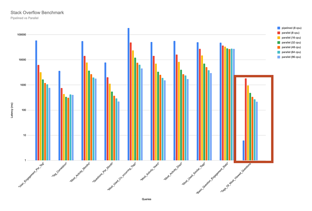
Luckily, this is data that we have readily available! More specifically, we have run these queries on machines with a CPU count ranging from 8 to 96 CPUs, and the results are impressive. (Note the scale on the Y-axis is logarithmic in the charts below).
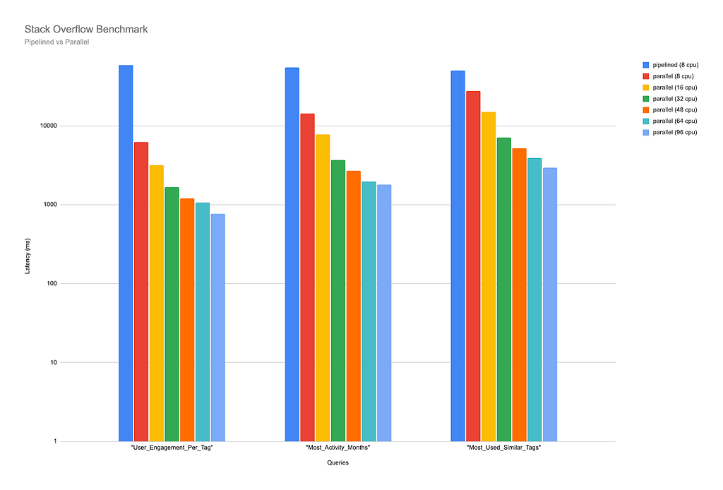
As this chart shows, the time taken for these queries to complete when run on parallel runtime reduces significantly as the number of CPUs increases. Our first query (which matches the graph for patterns in user activity on Stack Overflow) took just over 56,200 milliseconds to complete when run on pipelined runtime on a machine with 8 CPUs (remember that pipelined runtime will only use one core per query, even if more are available).
With the same CPU count, parallel runtime cuts the query time to 16,037 milliseconds. By the time we run it on a machine with 96 CPUs available, the query completion time is further reduced to just over 1714 milliseconds — more than 30 times faster than when run on pipelined runtime with 8 CPUs!
We ran several other queries, and, again, the trend is clear: the more CPUs available, the faster a query will complete when run on parallel runtime.
Note on concurrency
Perhaps it goes without saying, but the performance of parallel runtime is dependent on the concurrency of the database. In order for queries to benefit from it, it is not enough to have a lot of CPUs on a server. Those CPUs also have to be available for parallel runtime threads to use. In other words, queries that may be ideal to use with parallel runtime may not see their benefit if they are run against a high-concurrency database where the CPUs are already occupied by other queries.
Also note that because multiple threads are concurrently active when using parallel runtime, queries may require more heap memory.
Don’t forget about Pipelined!
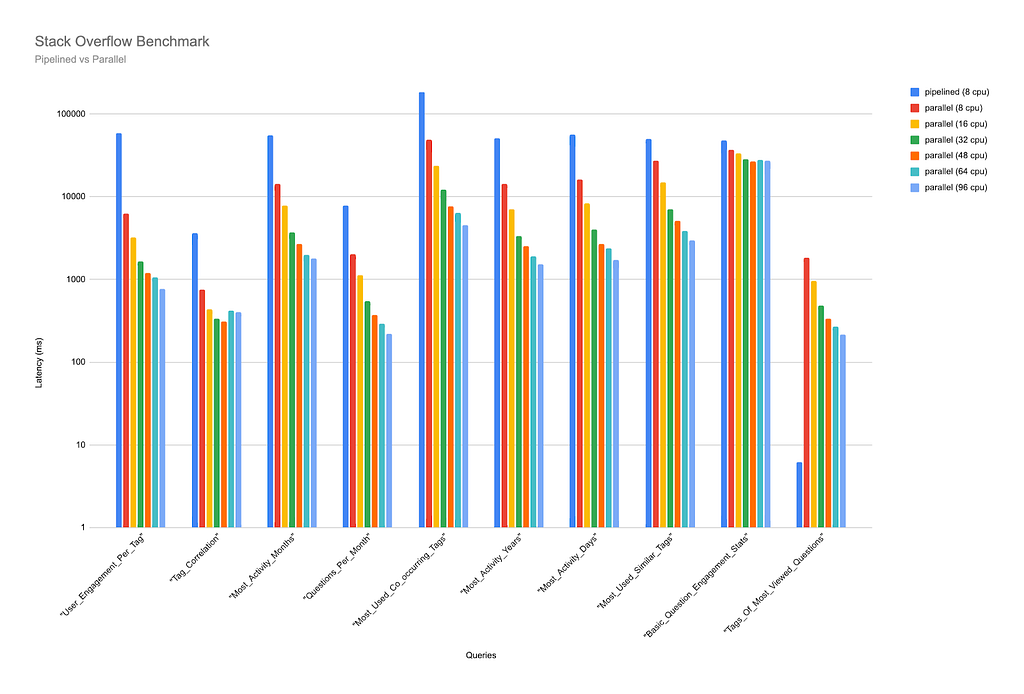
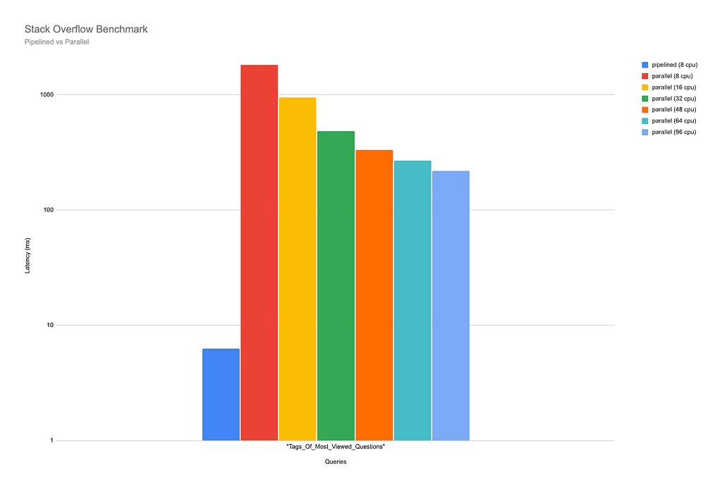
The observant reader might have spotted an anomaly in the above benchmarking results:
This query clearly did not benefit from being run on parallel runtime. In fact, while running it on pipelined runtime the query completed in just over 6 milliseconds, it took 1817 milliseconds to complete on parallel runtime with 8 CPUs available, and almost 219 milliseconds when run with 96 CPUs — still almost 40 times slower than when run on pipelined runtime. The results for each CPU count used in the benchmark can be seen more clearly below:
To explain why this is the case, we need to first take a look at the query, which matches the graph for the tags most commonly used on the most viewed questions in the Stack Overflow database:
MATCH (q:Question)
WITH q
ORDER BY q.views DESC
LIMIT 1000
MATCH (q)-[:TAGGED]->(t:Tag)
RETURN t.name AS tag, count(*) AS count
ORDER BY count DESC
LIMIT 10
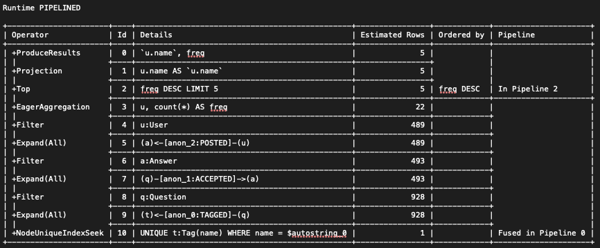
Then, we need to inspect the two plans produced by the different runtimes, and this time we start with parallel runtime plan:
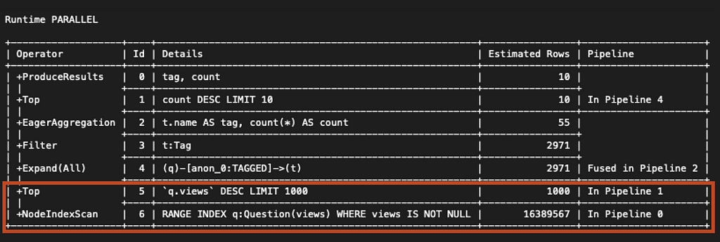
The reason why the parallel runtime is relatively slow to complete this query can be found in the first two operators in the plan. The first operator, NodeIndexScan, returns all (16,389,567) nodes with the Question label that have a views property. Those nodes are then sorted by the Top operator, and the top 1000 are returned.
By contrast, in pipelined runtime, we see that NodeIndexScan only returns 1000 rows, and the Top operator has been replaced by Limit.
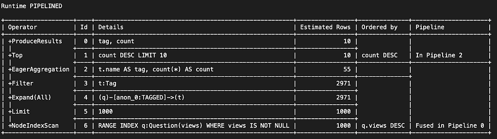
This is because pipelined runtime is able to leverage (i.e., reuse) the row order returned by the scan, which means that no sorting is necessary (notice the Ordered Bycolumn in the plan derived from pipelined runtime, which is not present in that generated by parallel runtime). More importantly, it means that only 1000 rows need to be read from the index.
Parallel runtime is not yet capable of leveraging index order, and as a result, the query is significantly faster on the pipelined runtime. There are other areas where parallel runtime may not be suitable.
The most obvious is any write statement, which is currently not supported by parallel runtime. Another area is graph-local queries, which only traverse a small section of the graph, where the pipelined runtime may very well complete queries faster than parallel runtime, which has additional management overhead.
The pipelined runtime thus continues to shine in some of the areas that parallel runtime is not particularly well suited for.
In general, while parallel runtime is optimized for running relatively few graph-global queries on databases with a low number of concurrent users, pipelined runtime is ideal for high transactional workloads where large numbers of queries are run concurrently by many users on the same system.
Whatever the situation, it is important to remember that different queries can be run on different runtimes on the same database deployment, which allows you to customize your queries with the runtime most suitable to the particular workloads of their different queries.
Another important thing to remember is that Neo4j 5.13 sees the first public release of parallel runtime. Neo4j users can expect to see some of its current limitations relaxed in future releases, as well as the performance of the runtime improved further.
Takeaways and use cases
After this brief comparison of the pipelined and parallel runtimes, our conclusion should not be that parallel runtime is a straightforward replacement or upgrade to pipelined runtime.
Rather, they should be understood as mutually complementary runtimes, each excelling in areas where the other may not be ideal. It is, therefore, important for advanced users of Neo4j to familiarize themselves with the situations in which query performance will likely improve with parallel runtime.
To recap, parallel runtime will very likely improve query performance if the following two conditions are met:
- Graph-global read queries are constructed to target a large section of a graph.
- The server has more than one available CPU.
What, then, are the potential use cases for parallel runtime? The fact that this question is difficult to answer comprehensively without going into a long list of different tasks and professions is a testament to both the versatility and potential of Neo4j’s most recent runtime.
But, to not evade the question completely, users engaged in any kind of explorative work, such as investigative journalism or data analytics, will most likely see the speed of their queries substantially improved. In general, we recommend that any read query that takes longer than half a second to complete would be a good candidate for running with parallel runtime.
But the best way to see if parallel runtime suits your purposes is, of course, to try it out for yourself!
If you want to read more about the Cypher runtimes, visit the official Neo4j documentation.
Speed Up Your Queries With Neo4j’s New Parallel Runtime was originally published in Neo4j Developer Blog on Medium, where people are continuing the conversation by highlighting and responding to this story.
Share Article


Explore
Related Articles

Hybrid Search in Neo4j: Full-Text, Vectors, and Graph Topology with Cypher