SumoDB in Neo4j: Microsoft Fabric bridging Decades of Rikishi — Part 4

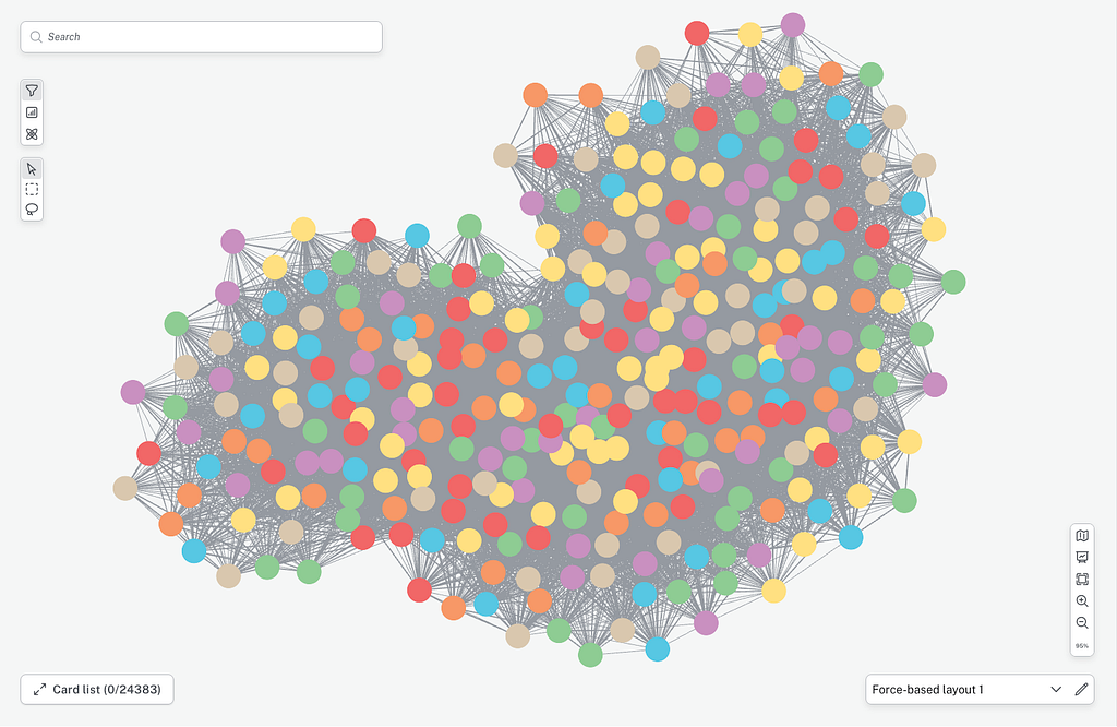
Nostalgia in sports is common — we often look back on previous generations with gilded lens. Ask any sumo fan whether the sport has changed and you’ll get the same answer: the big men don’t grapple like they used to. The belt battles that defined the 2000s have given way to shoving matches and quick pull-downs.

The first three parts of this series built a graph of professional sumo and used Neo4j to rank wrestlers by more than raw wins. Part 4 puts the claim to the test across 26 years of results, and it does the whole thing in Microsoft Fabric. The bout data lands in a Fabric Lakehouse, the graph algorithms run on Aura Graph Analytics, and the scored results flow straight back to OneLake where any Fabric tool can read them.

What we’re building

The pipeline has four hops, and each one hands off cleanly to the next:

sumo-api.com  →  Fabric Lakehouse (bronze → silver → gold)  →  Aura Graph Analytics  →  OneLake

The data comes from sumo-api.com, a free JSON API with Grand Sumo results back to 1958. We pull every bout from the top two divisions, Makuuchi and Juryo, for January 2000 through the present. That’s 78,710 bouts, roughly 47,000 in the top division and 31,000 in Juryo.

Why both divisions? Juryo is the proving ground where tomorrow’s champions learn their craft. Keeping it in lets us compare the two tiers and follow wrestlers as they climb from Juryo into top-division dominance, changing their style along the way.

From winning techniques to a style vector

Sumo records how every bout ends with a kimarite, the winning technique. There are 82 of them, from the workmanlike yorikiri (force-out) to the once-a-decade izori (backward body drop). Eighty-two categories are too many to reason about, so we group them into six style families:

Every wrestler gets a style vector: the share of their wins that came from each family. A pure pusher scores high on OSHI and near zero everywhere else. A belt technician loads up on YOTSU and NAGE. This vector is the raw material the graph clusters on.

The mapping is a plain Python dictionary, so it travels with every stage of the pipeline:

FAMILY = {
    "oshidashi": "OSHI", "tsukidashi": "OSHI",
    "yorikiri": "YOTSU", "tsuridashi": "YOTSU",
    "uwatenage": "NAGE", "shitatenage": "NAGE",
    "hatakikomi": "REACTIVE", "hikiotoshi": "REACTIVE",
    # ...82 techniques in total
}

Building the medallion in Fabric

Inside the Lakehouse we follow the standard bronze, silver, gold pattern. Bronze ingests the raw scrape and types the columns. Silver does the enrichment: it attaches the style family, parses rank classes, and assigns a prestige weight so that beating a yokozuna counts for more than beating a rank-and-file maegashira.

from pyspark.sql import functions as F
from itertools import chain

RANK_WEIGHT = {"Y": 6.0, "O": 5.0, "S": 4.0, "K": 3.0, "M": 1.0, "J": 0.5}
fam  = F.create_map([F.lit(x) for x in chain(*FAMILY.items())])
rank = F.create_map([F.lit(x) for x in chain(*RANK_WEIGHT.items())])
silver = (bronze
    .withColumn("kimarite_family",
                F.coalesce(fam[F.lower("kimarite")], F.lit("SPECIAL")))
    .withColumn("loser_rank_class", F.substring("loser_rank", 1, 1))
    .withColumn("loser_weight",
                F.coalesce(rank[F.col("loser_rank_class")], F.lit(0.5))))

Gold rolls the bouts up into the two tables the graph needs:

• gold_rikishi_style, one row per wrestler with the six style shares plus career stats. These become the Rikishi nodes.
• gold_defeated_edges, aggregated winner-to-loser pairs weighted by the prestige of the beaten opponent. These become the DEFEATED relationships.

We filter the node table to wrestlers with at least 20 top-two-division wins, which keeps the analysis on established careers with a stable style signal. That leaves a connected core of 317 wrestlers and 24,066 weighted edges.

Modeling the graph on Serverless AuraDB

Fabric ships a native way to turn Lakehouse tables into a graph. In your workspace, choose New item → Neo4j Graph Dataset, connect an AuraDB tenant, and pick Serverless so you can drive everything from a notebook.

When you create your Aura instance you will be given a set of credentials. Be sure to save these somewhere safe as you will need them again later.

Select the tables you wish to import into Neo4j. In our case we will only need our gold_rikishi_style table which will generate the nodes of the graph as well as the gold_defeated_edges table which will create the edges.

Neo4j Graph Intelligence importer uses AI to help generate potential graph model based on the tables you select. You can alter the model in the graph model editor or if everything looks right you can click Transform to graph.

After you press Transform to graph, the import job begins. You will see the steps processing as you wait.

When the job completes you will get notified both on screen and an email will be sent to your Fabric account email.Now you can navigate to Neo4j Graph in Fabric and query against it in Cypher through the query tab.

Running Aura Graph Analytics from a Fabric notebook

Now the fun part. Aura Graph Analytics gives you a serverless GDS session: you spin it up for the length of the job, run algorithms on a projected graph, write the answers back, and shut it down. The power of graphs an API call away in your notebooks.

Open a Python notebook in Fabric, install the client, and start a session against your AuraDB instance:

%pip install graphdatascience

from graphdatascience.session import (
    GdsSessions, AuraAPICredentials, DbmsConnectionInfo, AlgorithmCategory,
)
from datetime import timedelta
sessions = GdsSessions(api_credentials=AuraAPICredentials(CLIENT_ID, CLIENT_SECRET, TENANT_ID))
memory = sessions.estimate(
    node_count=1_000, relationship_count=30_000,
    algorithm_categories=[AlgorithmCategory.CENTRALITY,
                          AlgorithmCategory.COMMUNITY_DETECTION],
)
gds = sessions.get_or_create(
    "sumo-part4", memory=memory,
    db_connection=DbmsConnectionInfo(NEO4J_URI, NEO4J_USERNAME, NEO4J_PASSWORD),
    ttl=timedelta(hours=2),
)

Next, project the graph into the session. Its worth nothing a few things. We build the style vector inline from the six share properties and cast each one to a float, because a session graph rejects a list that mixes integers and floats. And we project the DEFEATED edge in reverse, from loser to winner, so that PageRank prestige flows toward the wrestlers who won the high-value bouts.

query = """
CALL () {
    MATCH (w:Rikishi)-[d:DEFEATED]->(l:Rikishi)
    RETURN l AS source, w AS target,
        { styleVector: [coalesce(toFloat(l.oshiShare),0.0), coalesce(toFloat(l.yotsuShare),0.0),
                        coalesce(toFloat(l.nageShare),0.0), coalesce(toFloat(l.reactiveShare),0.0),
                        coalesce(toFloat(l.legShare),0.0), coalesce(toFloat(l.specialShare),0.0)] }
            AS sourceNodeProperties,
        { styleVector: [coalesce(toFloat(w.oshiShare),0.0), coalesce(toFloat(w.yotsuShare),0.0),
                        coalesce(toFloat(w.nageShare),0.0), coalesce(toFloat(w.reactiveShare),0.0),
                        coalesce(toFloat(w.legShare),0.0), coalesce(toFloat(w.specialShare),0.0)] }
            AS targetNodeProperties,
        toFloat(d.weight) AS weight
}
RETURN gds.graph.project.remote(source, target, {
    sourceNodeLabels: labels(source), targetNodeLabels: labels(target),
    sourceNodeProperties: sourceNodeProperties, targetNodeProperties: targetNodeProperties,
    relationshipType: 'LOST_TO', relationshipProperties: { weight: weight }
})
"""
G, _ = gds.graph.project(graph_name="sumograph", query=query)

With the graph in memory, run two algorithms. Rank-weighted PageRank answers “who beat the strongest opposition,” and it writes a dominanceScore back to every wrestler:

gds.pageRank.write(
    G, relationshipTypes=["LOST_TO"], relationshipWeightProperty="weight",
    dampingFactor=0.85, maxIterations=30, writeProperty="dominanceScore",
)

This same algorithm can be run in the Bloom tab to show a visualization of which Rikishi are on top.

Then KNN builds a similarity graph from the style vectors. For each wrestler in the graph, the algorithm finds the top 15 wrestlers that have the closest similar style vector edges based on matches with other wrestlers and adds a score to those edges using Cosine Similarity. Louvain Community Detection then groups wrestlers who win the same way into style archetypes, this is done by maximizing the change in modularity as separate Rikishi are added to the same community:

gds.knn.mutate(
    G, nodeProperties={"styleVector": "COSINE"}, topK=15,
    similarityCutoff=0.80, randomSeed=42,
    mutateRelationshipType="SIMILAR", mutateProperty="score",
)
gds.louvain.write(
    G, relationshipTypes=["SIMILAR"], relationshipWeightProperty="score",
    writeProperty="styleArchetype",
)

This can be visualized in Bloom by selecting Rule-Based Color. We will first overlay the Primary Decade a Rikishi fought in and then show the Style Archetype they were found to have based on KNN & Louvain.

From a 10000 foot view it’s hard to tell if the overall archetypes have changed from one decade to the next. Lets write the results back to OneLake so we can do some SQL analysis to answer our starting question.

Writing results back to OneLake

The graph scores are useless if they stay locked in the session. Read them into a DataFrame and save them as a Delta table, and the whole of Fabric can query them:

df = gds.run_cypher("""
    MATCH (r:Rikishi)
    RETURN r.shikona AS shikona, r.primaryDecade AS decade,
           r.primaryDivision AS division, r.dominanceScore AS dominance,
           r.styleArchetype AS archetype,
           r.oshiShare AS oshi, r.yotsuShare AS yotsu,
           r.nageShare AS nage, r.reactiveShare AS reactive
""")
spark.createDataFrame(df).write.format("delta").mode("overwrite") \
     .saveAsTable("gold_rikishi_graph_scores")

From here the analysis is plain SQL, which means Power BI, notebooks, and the rest of your Fabric estate all read the same numbers.

What the graph found

Seven style archetypes

Louvain found seven communities, and their average style vectors give each a clear identity. The exemplars confirm them: the pushers really are the pushers.

The style mix shifts across decades

Track each archetype’s share of its decade and the fan’s hunch turns out to be half right. The belt-and-throw technician, the wrestler who wins with a grip and a throw the way Hakuho did, falls from 23% of the 2000s to about 16% of the 2010s and 2020s. Rising to meet it is the two-way hybrid, up from 11% to nearly 18%, now the most common archetype in the sport. Wrestlers are specializing less and mixing pushing with belt work more.

The aggregate technique counts tell the same story from another angle. In the top division, OSHI’s share of wins climbs from 25% in the 2000s to 32% in the 2020s, while throwing (NAGE) slips from 14% to 12%. Pushing is up, throwing is down, and the graph shows which wrestlers drove the change.

The shift reaches the very top

A change in the general population is one thing. The telling test is the leaderboard, so rank the most dominant wrestlers of each decade and read off their archetypes:

Three of the five most dominant men of the 2000s win with a grip and a throw. The belt still rules through the 2010s, the Hakuho decade. By the 2020s the leaderboard belongs to pushers and two-way hybrids, and Terunofuji stands out as the last belt specialist holding the top. The style drift runs the full length of the ranking, from the champions down to the rank and file.

The two divisions diverge

In the 2020s, Juryo leans more on belt work than Makuuchi does, with YOTSU about five points higher, while the top division shows more reactive sumo. The lower division is the more conservative, grappling-first tier, and wrestlers adapt as they climb. Follow a wrestler across the promotion line and many shift toward belt sumo when they reach the top: Asashoryu’s win mix gained 28 points of belt-and-throw share between his Juryo and Makuuchi careers.

Notes from the field

A few things will trip you up if you follow this path, so here’s what to watch for:

• The %pip install lasts one session. Fabric scopes it to the current Spark session, so rerun the install cell after any timeout or restart. For a permanent fix, bake graphdatascience into a custom Environment.
• Relative Lakehouse paths need a default lakehouse. If Files/… resolves to a trusted-service-user folder, you forgot to pin the lakehouse as default on that notebook.
• The tenant id is a bare UUID. Copy it out of the console URL and drop the trailing slash, or the session call fails with a project mismatch.
• The import tool renames columns. OSHI_share becomes oshiShare, total_wins becomes totalWins. Run db.propertyKeys() and match your Cypher to the real names.
• Session graphs want uniform lists. Wrap every style-vector element in toFloat(…) so a stray integer share doesn’t poison the list.

Building on your Own

The finished pipeline reads its data from OneLake, runs graph algorithms on a session that exists only while the job runs, and writes dominance scores and style archetypes right back to OneLake as a governed table. Your Fabric stack keeps its single source of truth, and it gains the one thing tables alone can’t give you: an understanding of how every wrestler connects to every other.

And the sport? The fans were onto something. Belt sumo hasn’t vanished, but the specialist who lived on the grip is giving ground to the wrestler who can do a bit of everything and shove when he needs to.

While Sumo wrestlers and their Kimarite style may not be your focus professionally, perhaps customers and their buying behavior is. This workflow could be analogously applied to customers buying or viewing habits across decades. Looking for similar customer archetypes and analyzing how the top customers are shifting and where.

You can run this yourself for free. Start a Serverless AuraDB instance and an Aura Graph Analytics session on the Neo4j console, point them at your own Fabric data, and see what your graph has been hiding.

---

SumoDB in Neo4j: Microsoft Fabric bridging Decades of Rikishi — Part 4 was originally published in Neo4j Developer Blog on Medium, where people are continuing the conversation by highlighting and responding to this story.