Clustering Large Graphs With CLARANS

Senior Data Scientist at Neo4j
13 min read

In a previous article, I discussed the benefits of using k-medoids to cluster graph data. In the k-medoids approach, you determine how many clusters you would like to partition the graph into. This number is called k. The algorithm identifies a set of k nodes in the graph called medoids. The other nodes in the graph are assigned to a cluster corresponding to whichever medoid they are closest to in the graph. The algorithm finds a set of medoids to minimize the sum of the distances between the nodes and their respective medoids.
The k-medoids approach offers several advantages for graph data. K-medoids can work with any distance metric as long as the metric can be used to assign a distance between all pairs of examples in the data set. For graph data, we can use the weighted or unweighted length of the shortest path between two nodes as the distance metric. This is an advantage over algorithms like k-means that most often use Euclidean distance. Euclidean distance doesn’t apply to graph topology without some transformation.
Another advantage of k-medoids is that the medoids returned by the algorithm can serve as typical examples for the clusters that they define. This makes the clustering results readily explainable to stakeholders.
An important drawback to some implementations k-medoids, such as the Partitioning Around Medoids (PAM) algorithm, is that they require that the distances between all pairs of nodes be calculated before running the algorithm. While Neo4j Graph Data Science includes the All Pairs Shortest Path algorithm, it is slow to run for graphs of more than a few thousand nodes.
This is where the CLARANS (Clustering Large Applications based on RANdomized Search) algorithm can be useful. Raymond T. Ng and Jiawei Han developed CLARANS to extend k-medoids to larger datasets than were practical with earlier k-medoid algorithms. Rather than exhaustively considering every node as a potential medoid, CLARANS randomly searches a subset of possible medoids. This means that we don’t have to calculate distances between all node pairs up front. We can calculate the distances as they are needed. We are able to arrive at a good approximation of the optimal solution while only calculating a fraction of the shortest paths in the graph.
The CLARANS Algorithm
Ng and Han described the steps of CLARANS as a graph problem. They imagined a graph where each node represents a set of k potential medoids. Nodes are related to each other in the candidate graph if they share all but one of their potential medoids in common. Since our underlying data is also a graph, I’ll refer to the underlying data as the “base graph” and the overlay of medoid candidate sets as the “candidate graph.”
At the start of the algorithm run, CLARANS picks an arbitrary node in the candidate graph to begin the search. This node is called the current candidate node. The algorithm calculates the distance from each base-graph node to its closest medoid. This total distance gives the current candidate a score.
CLARANS then begins checking the scores of randomly selected neighbors of the current candidate to see if they have a lower score than the current candidate. Each neighbor node has all but one of its medoids in common with the current candidate, so at this step, we are testing the effect of swapping out one medoid for another randomly selected medoid. As soon as we find a neighboring candidate node with a lower score, it becomes the current node, and we start searching its neighbors for a lower-scoring candidate. CLARANS includes a hyperparameter called maxneighbor. The algorithm counts the number of neighbors of the current candidate node that have been searched. If it does not find a node that improves the total distance score before the count reaches maxneighbor, then this iteration of the algorithm is complete.
Think of the CLARANS algorithm as a web crawler that is dropped into the candidate graph at a random node. It searches neighbors of that node until it finds one with a lower score. The crawler then moves to that neighbor and repeats the search until it can’t find a lower-scoring neighbor within the number of tries defined by maxneighbor. It is possible that the crawler could get stuck in a local minimum and miss out on lower scores in other parts of the graph. For this reason, CLARANS includes another hyperparameter called numlocal. This value indicates the number of times the algorithm will start at a random new position in the candidate graph. Having more than one starting point increases the probablity for the web surfers to find a value close to the global minimum score.
Implementing CLARANS in Python and Neo4j
The PyClustering library includes a Python implementation of CLARANS for tabular data. The project notebook for this blog demonstrates how we can use Neo4j Graph Data Science and the graph data science Python client to adapt CLARANS for graph data.
K-medoid algorithms assume we can calculate a distance from each node in the base graph to each medoid. This means that there must be a path from each node in the graph to each other node in the graph. If you have a disconnected graph, running weakly connected components (WCC) is a good first step towards clustering. After reviewing the results of WCC, you can use clustering algorithms like CLARANS to further analyze the structure of the largest WCC components.
The find_giant_component function creates a subgraph based on the largest connected component in the graph projection. It also applies a new label to the nodes in the largest component so that we can efficiently query these nodes with Cypher.
def find_giant_component(projection, wccProperty, subgraph_name, subgraph_node_label):
    # Mutate the graph with wcc id so we can use it for filtering
    gds.wcc.mutate(projection, mutateProperty=wccProperty)
    # Write the wcc id to the graph so we can use it for filtering in Bloom
    gds.graph.nodeProperties.write(projection, wccProperty)
    # Get the id of the giant component
    wcc_df = gds.graph.nodeProperties.stream(projection, wccProperty)
    biggest_component_id = wcc_df['propertyValue'].value_counts().idxmax()
    # Filter the projection to the giant component
    subgraph, result = gds.graph.filter(subgraph_name,
                                projection,
                                f"n.{wccProperty} = {biggest_component_id}",
                                "*")
    gds.run_cypher(f"""MATCH (n) WHERE n.wccId = $biggestComponentId
                       CALL apoc.create.addLabels(n, [$subgraphNodeLabel])
                       YIELD node
                       RETURN count(*) AS nodesUpdated""",
                  {"biggestComponentId": biggest_component_id,
                  "subgraphNodeLabel": subgraph_node_label})
    return subgraph, result, biggest_component_id
The function create_new_candidate randomly selects k nodes from the base graph to serve as a candidate set of medoids. This begins the search of the candidate graph. In order to create an audit trail of the search in the Neo4j database, we save the nodes of the candidate graph in Neo4j. Each candidate node is connected to the medoids within that candidate set by HAS_MEDOID relationships.
def create_new_candidate(k, label):
    candidate_df = gds.run_cypher(f"""MATCH (g:{label})
                                     WITH g ORDER BY rand()
                                     LIMIT $k
                                     WITH collect(g) AS medoids
                                     CREATE (c:Candidate)
                                     WITH c, medoids
                                     UNWIND medoids as m
                                     MERGE (c)-[:HAS_MEDOID]->(m)
                                     RETURN id(c) AS candidate_id
                                     LIMIT 1""",
                                  {"k":k, "label": label})
    return candidate_df.iloc[0,0]
The function calculate_candidate_cost calculates the distance from each medoid to all the nodes in the base graph. We calculate these distances using the Delta-Stepping Single-Source Shortest Path algorithm. This algorithm finds the shortest path from a node to all other reachable nodes in the graph. We create HAS_DISTANCE relationships between pairs of nodes in the base graph to record the length of these shortest paths in Neo4j. That way, we don’t have to recalculate them when a medoid is reused as part of a different candidate. This generates a lot of relationships in the graph, so your Neo4j instance will need some available storage space for this to run effectively.
Because our base graphs are undirected, the distance from node a to node b is the same as the distance from node b to node a. Neo4j’s implementation of Delta-Stepping Single-Source Shortest Path doesn’t give us an easy way to filter out target nodes where the HAS_DISTANCE relationship already exists in the other direction. This creates some redundant calculations, but in the test case I ran, less than 10% of the HAS_DISTANCE relationships that were created ended up being duplicates of existing relationships in the opposite direction.
Once we have calculated the distance from each medoid to the base nodes, we can determine which medoid is closest for each base node. The sum of the distances from the base nodes to the closest medoid becomes the score for this candidate set of medoids. The CLARANS paper describes a scoring mechanism that compares the distance from base nodes to their currently assigned medoid, the second closest medoid, and the swapped medoid. The Cypher statement in our function looks at the distance to all medoids associated with the candidate to find the closest medoid. This comparison is easier to express in Cypher than the comparison in the CLARANS paper. Our approach might be slightly less efficient than the approach in the CLARANS paper for large values of k.
def calculate_candidate_cost(projection, candidate_id):
    #If distances to all other nodes are not already present for each medoid,
    # calculate the missing distances
    gds.run_cypher("""
                      MATCH (c)-[:HAS_MEDOID]->(m)
                      WHERE id(c) = $candidateId
                      AND NOT EXISTS {(m)-[:HAS_DISTANCE]->()}
                      WITH m
                      CALL gds.allShortestPaths.delta.write(
                          $graphName,
                          {writeRelationshipType: "HAS_DISTANCE",
                          sourceNode: id(m)})
                      YIELD relationshipsWritten
                      RETURN relationshipsWritten
                          """,
                   {"candidateId": candidate_id,
                    "graphName": projection.name()})
    #Calculate the cost for this group of candidate medoids
    cost_df = gds.run_cypher("""
                      MATCH (c)-[:HAS_MEDOID]->(m)
                      WHERE id(c) = $candidateId
                      MATCH (m)-[d:HAS_DISTANCE]->(n)
                      WITH c, m, n, d
                      ORDER BY d.totalCost ASC
                      WITH c, n, collect(d.totalCost) AS costList
                      WITH c, n, costList[0] AS closestMedoidCost
                      WITH c, sum(closestMedoidCost) AS totalCost
                      SET c.totalCost = totalCost
                      RETURN totalCost""",
                  {"candidateId": candidate_id})
    return cost_df.iloc[0,0]
The create_neighboring_candidate function creates a neighboring candidate node for the current candidate in Neo4j. We create a HAS_NEIGHBOR relationship between the current candidate and the new candidate that is being created. That way we can retrace the steps of the search visually in Neo4j Bloom. You could implement CLARANS without this audit trail by keeping track of the current score and current set of medoids in Python.
def create_neighboring_candidate(candidate_id, k, label):
    new_candidate_df = gds.run_cypher(f"""
         MATCH (c:Candidate)
         WHERE id(c) = $candidateId
         MATCH (g:{label})
         WHERE NOT EXISTS {{(c)-[:HAS_MEDOID]->(g)}}
         WITH c, g
         ORDER BY rand()
         LIMIT 1
         MATCH (c)-[:HAS_MEDOID]->(m)
         WITH c, g, m
         ORDER BY rand()
         LIMIT $k -1
         WITH c, g, collect(m) AS medoids
         WITH c, medoids + g AS newMedoids
         CREATE (newCandidate:Candidate)
         WITH c, newCandidate, newMedoids
         MERGE (c)-[:HAS_NEIGHBOR]->(newCandidate)
         WITH newMedoids, newCandidate
         UNWIND newMedoids as newMedoid
         MERGE (newCandidate)-[:HAS_MEDOID]->(newMedoid)
         RETURN id(newCandidate) AS newCandidateId
         LIMIT 1""",
       {"candidateId": candidate_id,
        "k": k,
        "label": label})
    return new_candidate_df.iloc[0, 0]
The run_clarans function puts all the pieces together to run the CLARANS algorithm. You can pass in values for max_neighbor and num_local. If you do not, the function uses default values suggested in the CLARANS paper. Ng and Han found that a value of 2 for num_local was generally enough to get good results. A higher value caused the algorithm to run longer without improving the results very much in their experiments.
Each candidate node in the candidate graph has k(n – k) potential neighbors. This is because each of the k medoids in the candidate set could be swapped out for any of n – k other nodes in the base graph. The higher the percentage of these neighbors you search, the better your chance of getting close to the global minimum score. Ng and Han found through experimentation that searching between 1.25 and 1.5 percent of the total possible neighbors gave them a good balance between optimal results and fast run time. Our python implementation calculates max_neigbhor as 1.25% of the total possible neighbors if no value is specified when you call the function.
def run_clarans(projection, k, label, num_local=2, max_neighbor=None, verbose=False):
    #If max_neighbor was not provided, calculate 1.25% times k(n-k)
    if max_neighbor == None:
        node_count_df = gds.run_cypher(f"""MATCH (n:{label}) RETURN count(*) as nodeCount""")
        node_count = node_count_df.iloc[0,0]
        max_neighbor = round(k*(node_count-k)*0.0125)
        if verbose:
            print(f"max_neighbor: {max_neighbor}")
    min_cost = 999999999
    # The i counter keeps track of the number of times we begin the search at a new randomly selected candidate node
    i = 1
    while i <= num_local:
        current_candidate_id = create_new_candidate(k, label)
        current_cost = calculate_candidate_cost(projection, current_candidate_id)
        if verbose:
            print(f"Starting search from candidate {current_candidate_id} with cost {current_cost}")
        # The j counter keeps track of the number of times we have checked a neighbor of the currently selected node
        j = 1
        while j <= max_neighbor:
            neighbor_candidate_id = create_neighboring_candidate(current_candidate_id, k, label)
            neighbor_cost = calculate_candidate_cost(projection, neighbor_candidate_id)
            if verbose:
                print(f"Neighbor cost: {neighbor_cost}")
            if neighbor_cost < current_cost:
                j = 1
                current_candidate_id = neighbor_candidate_id
                current_cost = neighbor_cost
                if verbose:
                    print(f"Current cost: {current_cost}")
            else:
                j = j + 1
        if current_cost < min_cost:
            min_cost = current_cost
            best_candidate_id = current_candidate_id
            if verbose:
                print(f"Min cost: {min_cost}")
        i = i + 1
    return best_candidate_id, min_cost
Testing CLARANS on Two Graphs
I tested CLARANS on two graph datasets downloaded from The Network Data Repository with Interactive Graph Analytics and Visualization. The first dataset was a small genetics graph that I used in my previous k-medoids article. This dataset has 1,400 nodes and 1,600 relationships.
The second dataset is an author collaboration dataset. It has 12,000 nodes and 118,500 relationships.
I compared my graph-based CLARANS implementation with the FasterPAM k-medoid algorithm from the kmedoid Python package. The FasterPAM approach requires running All Pairs Shortest Path in Neo4j Graph Data Science to create a distance matrix representing all pairs of nodes in the graph.
Results on the Small Genetic Dataset
For the smaller genetic dataset, CLARANS with the default values for num_local and max_neighbors took about 249 seconds to run. The FasterPAM approach took 68 seconds, including the time to run All Pairs Shortest Path. The total distance score from FasterPAM was about 8% lower than the score from CLARANS. Since the FasterPAM approach took less time to run and gave a better score, it would definitely be the better algorithm to use for this dataset.
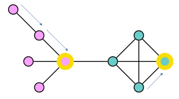
While the CLARANS result isn’t better than FasterPAM for this dataset, I still wanted to look at the CLARANS candidates in Neo4j Bloom because it clarifies how the algorithm works.
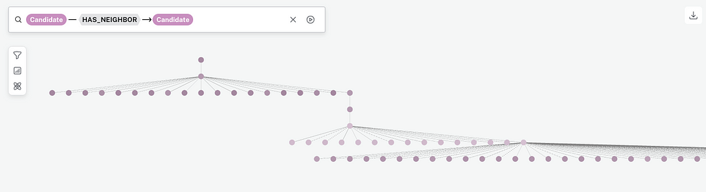
I set up a Bloom perspective that colors Candidate nodes based on their score. The darker the color, the higher (worse) the score. I used the hierarchical layout, so the first candidate searched shows at the top of the display, and later candidates show up lower. I searched for Candidate — HAS_NEIGHBOR-Candidate.
The segment of the full data visualization below shows one search beginning with a dark purple candidate at the top, moving to lighter nodes as the search progresses. At the bottom of the image, you can see that CLARANS checked many neighbors but didn’t find one with a lower score than the candidate on the right of the next to last row. In Bloom, you can right click and expand the HAS_MEDOID relationships for any of the Candidate nodes to see the associated medoids.
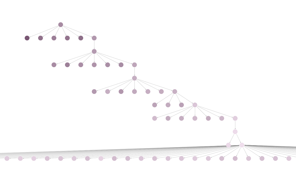
If you zoom out on the Bloom perspective, you will see two separate trees. This is because the num_local was set to two. The lowest scoring candidate across both searches was returned as the result.
Results on the Larger Author Collaboration Dataset
For the larger author collaboration dataset, the smallest Aura DS instance (8 GB memory, 2 CPU) did not have enough resources to run All Nodes Shortest Path. After upgrading an Aura DS instance two sizes larger (24 GB memory, 5 CPU), I was able to run All Nodes Shortest Path, but it took over 2.5 hours to complete. This was a big bottleneck to using the FasterPAM algorithm.
My CLARANS implementation was able to run successfully on the smallest Aura DS instance. After I upsized Aura DS to match the instance I used for FasterPAM, CLARANS completed in 23 minutes. The total distance score from CLARANS was less than 6% different from the FasterPAM score. If limited time or system resources prevent you from precomputing All Nodes Shortest Path for a graph of the size you are working with, CLARANS is a good alternative.
For the authors dataset, I found that CLARANS had been able to come up with its approximation of the optimal medoids by calculating 32% of the total possible shortest paths in the graph.
While some distances were calculated twice because of the limitations discussed in the description of the calculate_candidate_cost above, 90% of the distances were calculated only once. There is room for optimization by reducing these duplicate calculations, but they don’t appear to be a huge factor in overall performance.
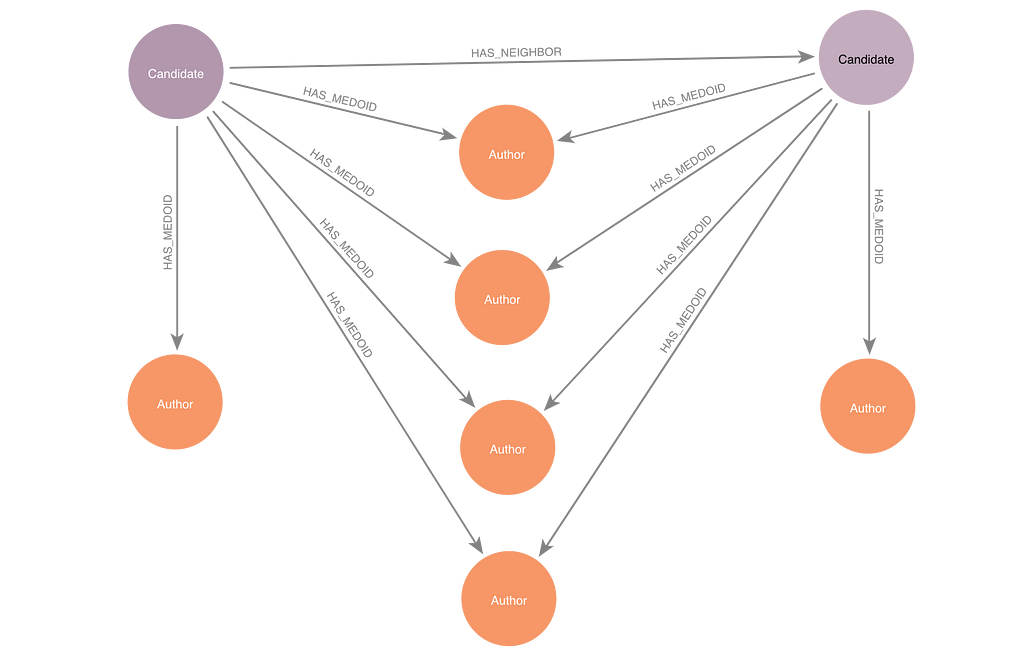
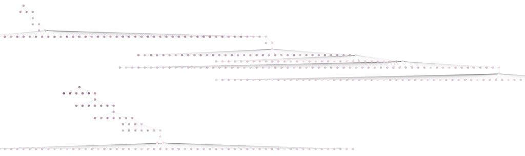
The Bloom visualization is harder to work with for the larger authors dataset than the smaller genetic dataset because max_neighbors is so much larger for the authors dataset. However, this close-up shows the detail of one of the trees.
Conclusion
Most Python implementations of k-medoid algorithms require pre-computation of distances between all pairs of items in the dataset. If the distance metric is easy to compute, like Euclidian distance, this pre-computation is not a bottleneck. However, when applying k-medoid algorithms to graph data, finding the shortest paths between all pairs of nodes can be very expensive.
CLARANS offers a way to discover medoids that are a good approximation of the optimum medoids by computing a relatively small percentage of the possible shortest paths in the graph. For medium and large graphs, the improvement in run time over other k-medoid approaches makes CLARANS a good choice.
Clustering Large Graphs With CLARANS was originally published in Neo4j Developer Blog on Medium, where people are continuing the conversation by highlighting and responding to this story.
Share Article


Explore
Related Articles


Text2Cypher Across Languages: Evaluating Foundational Models Beyond English