Graph and Lakehouse, Friends at Last

Getting Started With Neo4j Virtual Graph on Databricks

Mini Graph Tutorial | TPC-H Databricks Walkthrough | Complex Queries

If you work in a modern data lakehouse, your data is probably clean, well-governed, and sitting in Databricks. The problem is that relationships are implicit, often buried in foreign keys and join tables, which makes them hard to work with for humans and AI agents alike. It can be difficult for humans writing complex common table expressions (CTEs) to answer questions that should be straightforward. Agents either have to guess at the relationships or rely on prompt engineering to navigate them. What’s missing is a semantic-friendly surface that exposes the data in a way that’s natural to reason over.

Neo4j has a new answer to this: Neo4j Virtual Graph.

Introducing Neo4j Virtual Graph: Graph reasoning on the data you already have – Graph Database & Analytics

Virtual Graph gives your lakehouse data a graph model, where relationships become explicit first-class semantic citizens rather than something implied by a foreign key or hidden in a join table. Your schema stops looking like a collection of disconnected tables and starts looking like a real domain model, one that humans can navigate intuitively and AI agents can reason over without needing to know anything about the underlying physical structure.

And your data doesn’t have to move to gain this advantage. Virtual Graph sits on top of your existing Databricks lakehouse. Access is governed by Unity Catalog under the identity of the connection you configure. You query the Virtual Graph using Cypher statements that are translated to SQL, and executed on your existing compute with full predicate pushdown. No copy. No pipeline. No new system of record.

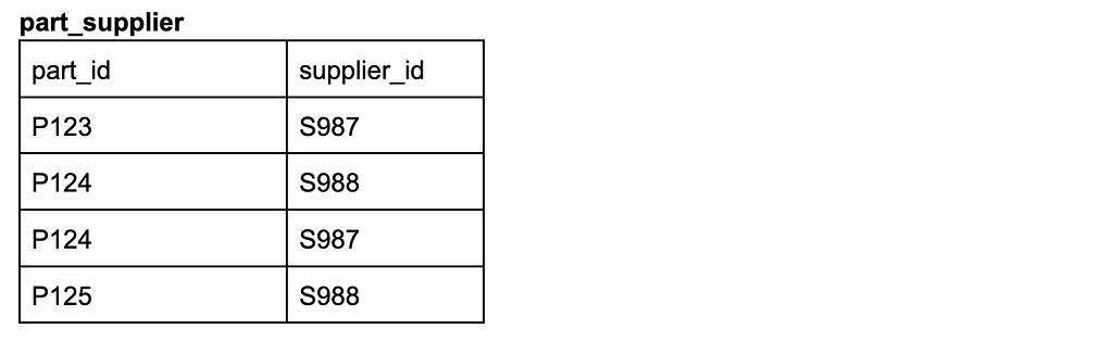
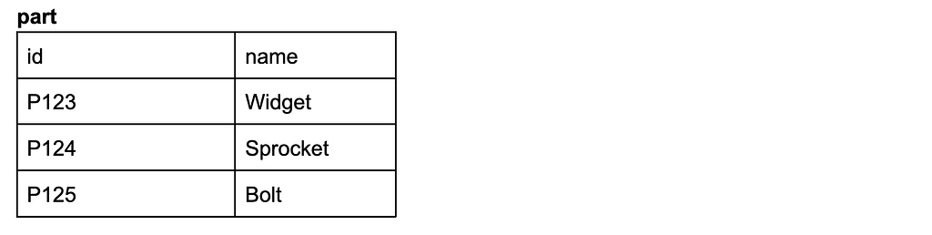
Let’s look at an example to see how it works. Consider a join table called part_supplier that is used to encode many-to-many relationships between part and supplier.

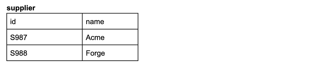
In a graph, you convert the join table into a relationship as shown in the following diagram.

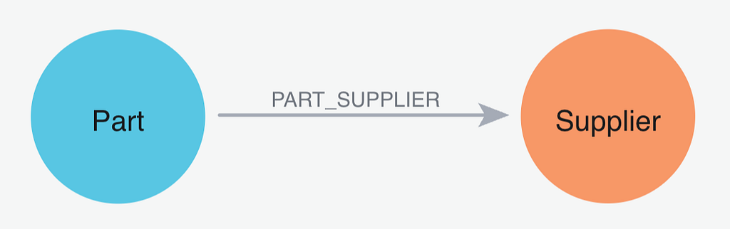
Written as a Cypher pattern, it becomes (:Part)-[:PART_SUPPLIER]->(:Supplier) where PART_SUPPLIER converts the part_supplier table into a first-class relationship. You can even pick a more semantically relevant name for the relationship. For instance, if your join table was cst_loc this could become a CUSTOMER_LOCATION relationship in in your graph model. When you define the model, you can choose new, business relevant terms in place of cryptic table names as you see fit.

Given this tiny graph model, the instance data in the table above would look like this in the graph:

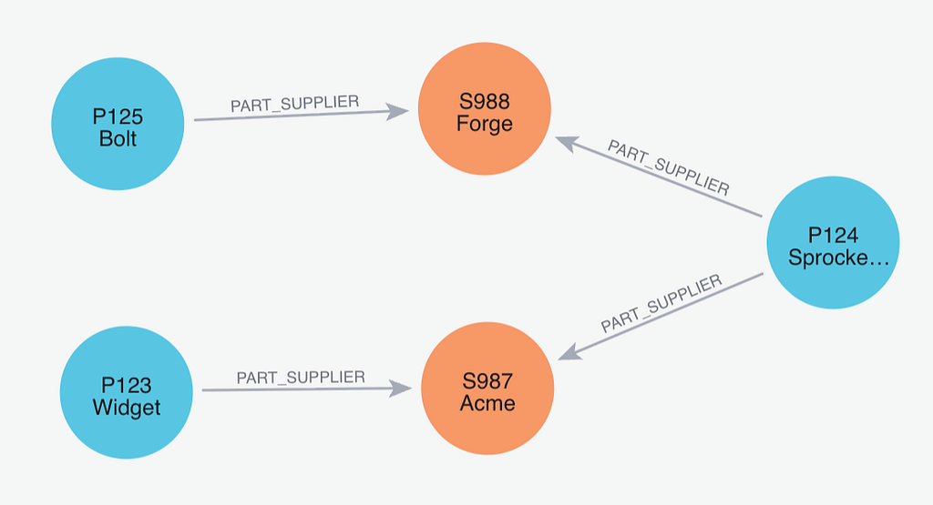
Which enables you to immediately see that 1 part is made by two suppliers, and each supplier makes 2 parts. This information is often difficult to see when looking at ids and mentally trying to connect the dots.

But the real power comes from simplified, more intuitive ways to query the data. Retrieving the part id, part name, and supplier name in SQL would look like this:

SELECT ps.part_id, p.name AS part_name, s.name AS supplier_name
FROM part_supplier ps
JOIN part p ON ps.part_id = p.id
JOIN supplier s ON ps.supplier_id = s.id

Where in Cypher the query looks like this:

MATCH (p:Part)-[:PART_SUPPLIER]->(s:Supplier)
RETURN p.id AS partId, p.name AS partName, s.name AS supplierName

The JOINs are now explicit relationships and very similar to natural language. Who are the part suppliers? (:Part)-[:PART_SUPPLIER]->(:Supplier) . It’s obvious and uses business language.

This matters especially when you’re building agentic workflows. A large language model (LLM) generating Cypher queries against Virtual Graph only needs the graph schema: node labels, relationship types, property names and types. It doesn’t need to know Databricks table names, foreign-key column names, or join logic.

The graph schema becomes business level a natural language interface to the warehouse. And because every Cypher statement is translated into SQL deterministically, by a fixed translator and not an LLM, results stay reproducible and auditable: the LLM (or human) proposes the Cypher query, the engine guarantees the execution.

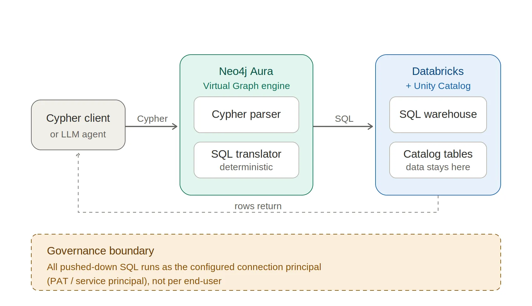
Let’s take a look at the end-to-end architecture. As shown in the diagram below, we have a Cypher client that talks to the Virtual Graph Engine in Aura. The Cypher query is parsed and translated into SQL via a deterministic SQL translator. The generated SQL statement is pushed down to Databricks compute, with data staying in Unity Catalog and the identity boundary marked. During initial setup, the connection between the Virtual Graph and Databricks is made using a Databricks developer access token, so the SQL statement executing in Databricks has the same security restrictions as the developer access token.

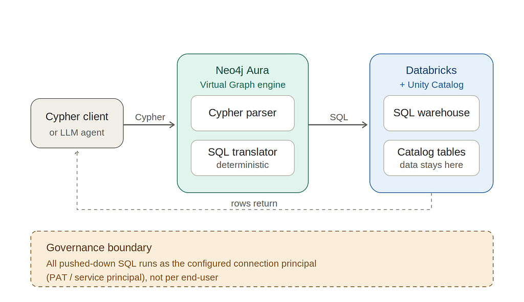
You can read the full motivations and architecture in the official announcement. In this post, I’m going to walk through setting up a Virtual Graph on top of Databricks and show some query patterns that demonstrate its utility for simplifying complex questions.

Here’s a preview. This query answers “what is the total net revenue by region and market segment?” A question that requires a 4-table JOIN and GROUP BY in SQL, written as a graph traversal that makes it clear what data we are getting and how it’s related:

MATCH (r:Region)<-[:IN_REGION]-(n:Nation)<-[:CUSTOMER_LOCATION]-(c:Customer)
  -[:ORDER]->(o:Order)-[:LINE_ITEM]->(l:LineItem)
RETURN r.name AS region, c.marketSegment AS segment,
  count(DISTINCT o.id) AS orders,
  count(l) AS lineItems,
  sum(l.extendedPrice * (1 - l.discount)) AS netRevenue
ORDER BY netRevenue DESC

Note: Cypher ignores spaces between pattern elements so even though -[:ORDER]-> is on the next line its still connected to Customer, i.e. …before…-(c:Customer)-[:ORDER]->(o:Order)->…after…

Cypher: You can do it too!

You might be thinking. I don’t know Cypher. I know SQL. The good news is that basic Cypher is really easy to learn, and there are a lot of similarities between Cypher and SQL. The primary difference is specifying MATCH patterns. Keywords such as WHERE and RETURN are almost exactly the same.

Let’s look at a MATCH pattern.

(c:Customer)-[:ORDER]->(o:Order)-[:LINE_ITEM]->(l:LineItem)

First you’ll notice that we have ASCII art patterns where parentheses ( ) specify a node pattern, and brackets [ ] specify a relationship pattern.

What are nodes really? Nodes are essentially table rows, i.e. entities in your domain. There is an old Neo4j slogan called Tables to Labels. This means you can think of a Table name as a Label. By convention, Node Labels are typically capital CamelCase and so the table name customer translates to the node label Customer.

Since a table name is a node label, then a node is equivalent to a table row.

If we had a customer table with 1 row:

Then that directly corresponds to a node:

(:Customer {id: ‘C456’, name: ‘Alice’})

Where Customer is the node’s label, id and name are the node’s property keys, and C456 and Alice are the associated property values.

Neo4j is known as a Labeled Property Graph, or LPG, which means:

• Graph: a data structure where nodes are connected to each other via relationships (nodes are sometimes called vertices and relationships are sometimes called edges)
• Labeled: each node can have 1 or more labels, like Customer
• Property: nodes and relationships can have key/value properties

The table columns id and name were translated to node properties, which in Cypher can be accessed via an inline node pattern (:MyLabel {key: value}) using braces { }, or by referencing them using dot syntax on variables.

In a MATCH pattern we can find Alice by customer id like this:

MATCH (c:Customer)
WHERE c.id = 'C456'
RETURN c.name

When working with node and relationship patterns, you can specify a variable, in this case c, which you can use later in the statement.

For relationships, we use an arrow syntax ()–>() which follows the direction of the arrow in the defined graph model. Before we talk more about relationships, let’s investigate graph modeling.

Graph Modeling and Mapping to SQL Schema

The graph model specifies how tables and their foreign key relationships map into graph nodes and relationships. These are the high level mappings:

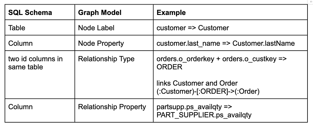
When you build your graph model, you can choose your own names for Node Labels, Relationship Types, and Property Names. It’s best practice to choose terminology that is understandable to business users who work in the domain. Choosing terminology that captures the business semantics (meaning) creates an easy surface for both human users and AI agents alike.

We’ll set up a graph model when we walk through the scenario, but for now let’s look at this small model linking Customer to Order and Nation. Customer is linked to Order via the ORDER relationship type, and linked to Nation via the CUSTOMER_LOCATION relationship type.

I say relationship type instead of relationship because this is the model level, and we aren’t dealing with instance data yet.

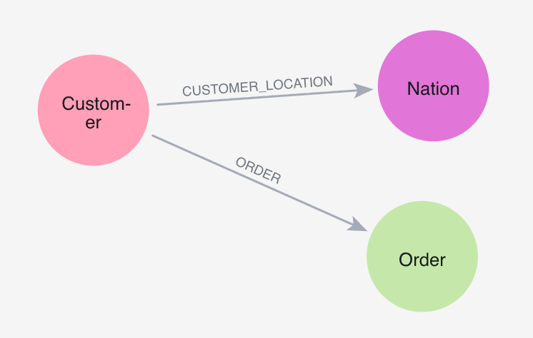
We’ll use this very small model to circle back to how relationships are used in Cypher MATCH statements.

Traversing Relationships in Cypher

Now that we have our model, we can see how MATCH patterns work when we use relationships. The actual nodes and relationships that correspond to the model look like this:

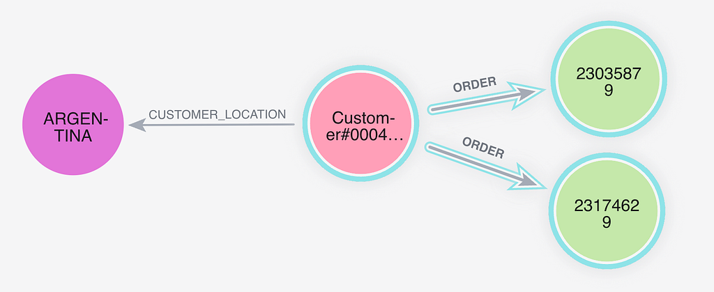
Where we have Customer with a name property value of Customer#000412510 linked to:

• a Nation with a name property value of ARGENTINA via the CUSTOMER_LOCATION relationship
• two Order nodes with id property values of 23035879 and 23174629 via ORDER relationships

Note: name and id have been configured as display properties

We can match the highlighted nodes and relationships by specifying this query:

MATCH (c:Customer {name:'Customer#000412510'})-[r:ORDER]->(o:Order)
RETURN c.name, o.id

Which returns this result:

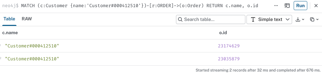
To look for customer orders, you specify the relationship type you want to traverse over and the query follows all paths that match that pattern. Since we specified ORDER it followed ORDER relationships only and not CUSTOMER_LOCATION. If you want both relationships you could either omit the relationship type or add them both separated by a pipe |. Given our model, all of these would do the same thing:

• -[r:ORDER|CUSTOMER_LOCATION]->
• -[]->
• –>

The great news is that if you ever want to see how the Cypher is translated into SQL, you can use the EXPLAIN keyword.

EXPLAIN MATCH (c:Customer {name:'Customer#000412510'})-[r:ORDER]->(o:Order)
RETURN c.name, o.id

You will see the full query plan and how it translated the Cypher to SQL. This should be useful both from an understanding and troubleshooting perspective. The SQL for the query above is:

SELECT `c`.`c_name` AS `c_name`, `o`.`o_orderkey` AS `o_id` 
FROM `tpch_vg`.`customer` AS `c` 
JOIN `tpch_vg`.`orders` AS `r` ON `r`.`o_custkey` = `c`.`c_custkey` 
JOIN `tpch_vg`.`orders` AS `o` ON `o`.`o_orderkey` = `r`.`o_orderkey` 
WHERE (`c`.`c_name` = ? /*autostring0*/)

The query is parameterized using /*autostring0*/, which takes the value ‘Customer#000412510’. Parameter binding (the bind variable shown as /*autostring0*/) is what prevents SQL injection. The backticks around identifiers are separate: they safely quote table and column names.

Now that you have a good understanding of Cypher, modeling, and how it translates to SQL let’s walk through a full example.

The Dataset: TPC-H on Databricks

For this walkthrough I’m using TPC-H, the classic supply chain benchmark dataset that ships natively in every Databricks Unity Catalog workspace under samples.tpch. It’s an eight-table schema covering orders, customers, line items, suppliers, parts, and their regional hierarchies. It’s complex enough to write interesting queries, familiar enough that the domain is self-explanatory, and readily available without any setup (almost).

One thing you’ll need to be aware of up-front: Virtual Graph currently requires each node to have a single-column ID, and TPC-H’s lineitem table uses a composite primary key (l_orderkey + l_linenumber). I’ll show the workaround in the setup steps.

Setting Up Virtual Graph on Databricks

What you’ll need:

• A Neo4j Aura account (console.neo4j.io)
• A Databricks workspace with Unity Catalog enabled
• The samples.tpch catalog (included in all Databricks workspaces by default)

The full setup guide is in the Neo4j Virtual Graph docs. Here are the setup steps working with the sample catalog.

Step 1: Copy the TPC-H Tables Into Your Own Schema

Schema samples.tpch is read-only, so you’ll need to copy the tables into a schema you own. This is also where you fix the composite key issue, so we’ll need to do this in order to import lineitem so it can work in the Virtual Graph. You’ll need to replace my_catalog with the name of the Databricks catalog you’ll be working with.

First, create a target schema:

CREATE SCHEMA IF NOT EXISTS my_catalog.tpch_vg;

For the small reference tables, DEEP CLONE is the fastest option:

CREATE OR REPLACE TABLE my_catalog.tpch_vg.nation
DEEP CLONE samples.tpch.nation;

CREATE OR REPLACE TABLE my_catalog.tpch_vg.region
DEEP CLONE samples.tpch.region;

For the transactional tables, I’d recommend copying a referentially consistent 1M-row slice anchored on lineitem. This avoids orphaned nodes in the graph while keeping the dataset manageable:

-- Start with 1M lineitems
CREATE OR REPLACE TABLE my_catalog.tpch_vg.lineitem AS
SELECT * FROM samples.tpch.lineitem LIMIT 1000000;

-- Pull only the orders referenced by those lineitems
CREATE OR REPLACE TABLE my_catalog.tpch_vg.orders AS
SELECT DISTINCT o.* FROM samples.tpch.orders o
INNER JOIN my_catalog.tpch_vg.lineitem l ON o.o_orderkey = l.l_orderkey;

-- Customers referenced by those orders
CREATE OR REPLACE TABLE my_catalog.tpch_vg.customer AS
SELECT DISTINCT c.* FROM samples.tpch.customer c
INNER JOIN my_catalog.tpch_vg.orders o ON c.c_custkey = o.o_custkey;

-- Suppliers and parts referenced by those lineitems
CREATE OR REPLACE TABLE my_catalog.tpch_vg.supplier AS
SELECT DISTINCT s.* FROM samples.tpch.supplier s
INNER JOIN my_catalog.tpch_vg.lineitem l ON s.s_suppkey = l.l_suppkey;

CREATE OR REPLACE TABLE my_catalog.tpch_vg.part AS
SELECT DISTINCT p.* FROM samples.tpch.part p
INNER JOIN my_catalog.tpch_vg.lineitem l ON p.p_partkey = l.l_partkey;

CREATE OR REPLACE TABLE my_catalog.tpch_vg.partsupp AS
SELECT DISTINCT ps.* FROM samples.tpch.partsupp ps
INNER JOIN my_catalog.tpch_vg.lineitem l
ON ps.ps_partkey = l.l_partkey AND ps.ps_suppkey = l.l_suppkey;

1M lineitems gives you roughly 200–250k orders, 150k customers, and a proportionate slice of parts and suppliers. More than enough for us to showcase the capabilities of the Virtual Graph.

Step 2: Fix the Composite Key on lineitem

Virtual Graph needs a single column to use as the node ID. lineitem doesn’t have one; it uses l_orderkey + l_linenumber together as the key. The fix is a generated column:

ALTER TABLE neo4j_graph_engine.tpch_vg2.lineitem
ADD COLUMN lineitem_id STRING;

UPDATE neo4j_graph_engine.tpch_vg2.lineitem
SET lineitem_id = CONCAT(CAST(l_orderkey AS STRING), '_', CAST(l_linenumber AS STRING));

OPTIMIZE neo4j_graph_engine.tpch_vg2.lineitem;

This adds a stable, unique string ID called lineitem_id per row without touching the underlying data. From Virtual Graph’s perspective, it looks like any other column.

This is the main schema-level gotcha when bringing an existing warehouse schema into Virtual Graph. Any table with a composite primary key needs a single-column identifier (the generated column above is an identifier, not a primary key). Keep it in mind when you’re mapping your own schemas.

Step 3: Create a Virtual Graph

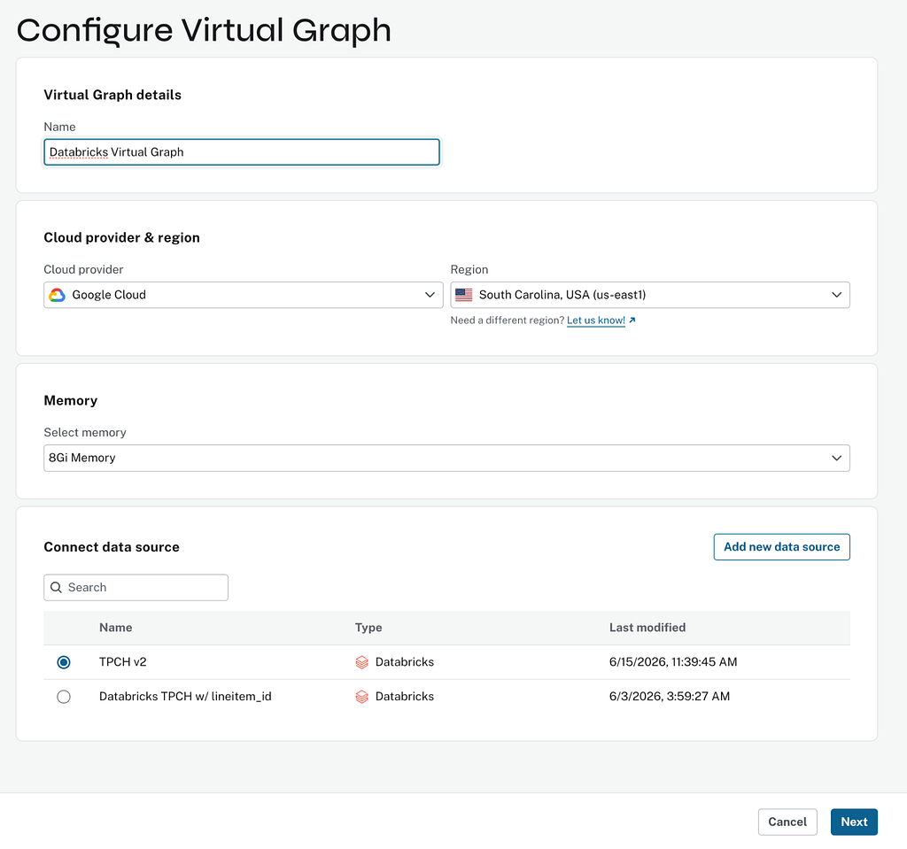
From the Aura console, navigate to Virtual Graphs and click Create Virtual Graph. You’ll need to enter a Name and select a Cloud Provider and Memory. If this is the first time you’re creating a Virtual Graph, you’ll need to click Add new data source (See Step 4). Once you have a data source, you’ll click Next.

The diagram below shows the form filled out with Google Cloud as the cloud provider and 8 GB of Memory.

Step 4: Connect Virtual Graph to Databricks

Once you’ve clicked Add new data source you’ll see an Add data source popup. Select Databricks. The following popup will appear:

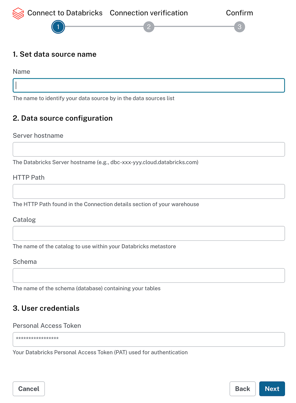
Enter a Name, then fill out the form using the following guidance:

The Server hostname

• dbc-xxxxxxxx-yyyy.cloud.databricks.com
• from SQL Warehouses > Connection Details in Databricks

The HTTP Path

• /sql/1.0/warehouses/xxxxxxxxxxxxxxxx
• from SQL Warehouses > Connection Details in Databricks

Your catalog

• my_catalog
• the name of your Databricks catalog

Your schema name

• tpch_vg
• the name of the schema we created in Step 1

A personal access token or service principal

• This token is how access is governed by Unity Catalog
• from User > Settings > Developer > Access Tokens in Databricks

Important: Make sure the user associated with this token has sufficient privileges to read the schema and execute queries against your schema

Once the connection is established, you will be presented with a preview screen showing the connection information along with the discovered tables and columns. Click Confirm to proceed.

Step 5: Create the Graph Model

Click on Create new model and click Next. You’ll see an option to generate your data model in three different ways: Define Manually, Generate from Schema, Generate with AI. Select Generate with AI.

Information from the schema is used to generate a property graph model automatically. This is where the semantic lift happens: foreign-key relationships become edges, join tables become relationship types with properties.

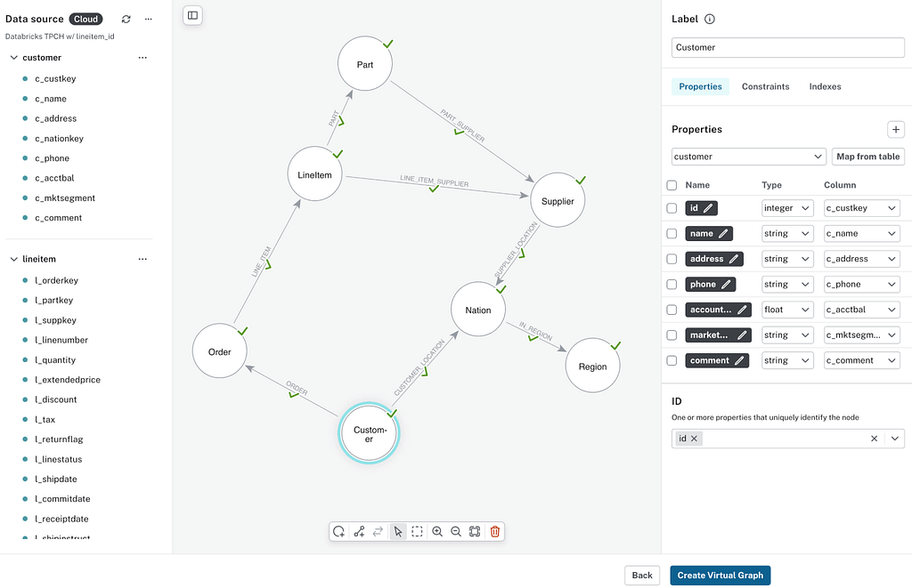
The left-hand side shows the Databricks schema, the middle part shows the graph model, and the right shows the property mappings based on the highlighted item in the graph model.

For TPC-H, the model looks like this:

(:Customer)-[:CUSTOMER_LOCATION]->(:Nation)
(:Customer)-[:ORDER]->(:Order)
(:Order)-[:LINE_ITEM]->(:LineItem)
(:LineItem)-[:LINE_ITEM_SUPPLIER]->(:Supplier)
(:LineItem)-[:PART]->(:Part)
(:Part)-[:PART_SUPPLIER {ps_availqty, ps_supplycost}]->(:Supplier)
(:Supplier)-[:SUPPLIER_LOCATION]->(:Nation)
(:Nation)-[:IN_REGION]->(:Region)

Important: Assuming you’ve used the Auto-Generated model, the names and directions of the relationships might be different. To follow along, you should ensure that all of the names in your graph model match the ones above, and that the relationship directions all point the correct way. You can select a Label or Relationship Type to show it in the right hand pane. There you can change the name or relationship direction.

When you’re developing your own model, you can pick names and directions as appropriate, but it’s important that they match for this article since the Cypher statements we will write depend on the exact name and directions. The same applies to property names: the queries below use friendly names such as name, id, marketSegment, extendedPrice and discount. If your auto-generated model still shows raw column names (c_name, o_orderkey, and so on), rename the properties to match before running the queries, or the queries will error.

Doubly Important: When you are defining your own graph model for virtual graphs it is important that each RELATIONSHIP_TYPE you define is unique. This is a current limitation of the Virtual Graph model mapping. The model above uses unique relationship names.

Once you’ve edited the model to match the names and directions above, click Create Virtual Graph to finish the process. You’ll be asked to download the connection information. Do this and proceed. It may take a few minutes for the Virtual Graph to be created.

Step 6: Run Your First Query

Connect to the Virtual Graph using the Query tool in the Aura console and then run this query to verify it’s working:

MATCH (c:Customer)-[:ORDER]->(o:Order)
RETURN c.name, count(o) AS orderCount
ORDER BY orderCount DESC
LIMIT 10

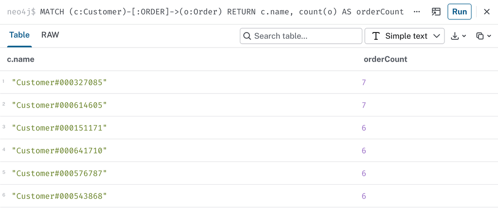
If you see results, you have a working Virtual Graph over live Databricks data.

The Power of Virtual Graphs: Complexity made Easy

Now for the interesting part. We’ll walk through some more complex scenarios so you can see how viewing your Databricks SQL Catalog as a graph model can help you answer complex questions.

Star Schema Navigation: Revenue by Region and Segment

The TPC-H schema is a textbook star: Order is the fact, Customer, Nation, Region, and LineItem are dimensions. In SQL this is a 4-way JOIN with a GROUP BY. In Cypher it’s clear we’re traversing from Region through Customer all the way to LineItem and computing aggregations.

MATCH (r:Region)<-[:IN_REGION]-(n:Nation)<-[:CUSTOMER_LOCATION]
  -(c:Customer)-[:ORDER]->(o:Order)-[:LINE_ITEM]->(l:LineItem)
RETURN r.name AS region, c.marketSegment AS segment,
  count(DISTINCT o.id) AS orders,
  count(l) AS lineItems,
  sum(l.extendedPrice * (1 - l.discount)) AS netRevenue
ORDER BY netRevenue DESC

Fixed-depth traversals like this are Virtual Graph’s sweet spot. The Cypher pattern and the SQL execution plan line up closely: the MATCH clause becomes an equivalent multi-table JOIN (sometimes with an extra self-join, where a relationship and its target node map to the same table).

Bipartite Intersection: Cross-Regional Supplier Reach

This one’s harder to express in SQL. The question is: which suppliers are serving customers in more than one region? That’s a bipartite graph intersection, finding entities that appear on both sides of a many-to-many relationship filtered by a dimension. In SQL it needs a self-join common table expression (CTE). In Cypher:

MATCH (o:Order)<-[:ORDER]-(c:Customer)-[:CUSTOMER_LOCATION]->
  (cn:Nation)-[:IN_REGION]->(cr:Region)
MATCH (o)-[:LINE_ITEM]->(l:LineItem)-[:LINE_ITEM_SUPPLIER]->
  (s:Supplier)-[:SUPPLIER_LOCATION]->(sn:Nation)-[:IN_REGION]->(sr:Region)
WITH s.name AS supplier, sr.name AS supplierRegion,
  collect(DISTINCT cr.name) AS customerRegions
WITH supplier, supplierRegion, customerRegions,
  size(customerRegions) AS regionCount
RETURN supplier, supplierRegion, customerRegions, regionCount
ORDER BY regionCount DESC
LIMIT 20

One thing worth calling out: the second MATCH anchors on o from the first pattern. That’s on purpose. If you start from Supplier independently and work toward Customer in separate MATCH clauses without connecting them, you get a cardinality explosion before the WITH has a chance to reduce. In Virtual Graph, as in native Neo4j, it’s useful to think about how the data is being accessed, and using the EXPLAIN keyword can help you optimize your queries.

Parametric Lookup: Agent and Text2Cypher Ready

One of the most compelling uses for Virtual Graph is as a query target for agentic workflows. The reason: an LLM generating Cypher only needs the graph schema. It doesn’t need to know Databricks table names, foreign-key columns, or join logic. The graph schema acts as a semantic interface to the warehouse.

:params { customerName: "Customer#000286435" }

MATCH (c:Customer)-[:ORDER]->(o:Order)-[:LINE_ITEM]->
  (l:LineItem)-[:PART]->(p:Part)
WHERE c.name = $customerName
RETURN c.name AS customer, o.id AS orderId, o.orderDate,
  o.orderStatus, p.name AS part,
  l.quantity, l.extendedPrice, l.discount, l.shipDate
ORDER BY o.orderDate DESC
LIMIT 50

The 3-hop traversal becomes a 4-table JOIN. This pattern works reliably, returns structured results, and is exactly the kind of query an LLM can generate from schema alone.

Multi-Role Supplier Scoring

Virtual Graph can score entities by their participation across multiple relationship types, something that’s genuinely awkward to compute in SQL without dedicated pipeline work.

The question: which suppliers in Europe are both listed in the parts catalogue and actively fulfilling orders? A supplier that appears in both roles is more operationally central than one that’s catalogue-only.

MATCH (s:Supplier)-[:SUPPLIER_LOCATION]->(:Nation)
  -[:IN_REGION]->(:Region {name: "EUROPE"})
MATCH (s)<-[:LINE_ITEM_SUPPLIER]-(lineItem:LineItem)
  -[:PART]->(part:Part)-[:PART_SUPPLIER]->(s)
WITH s.name AS supplier,
  size(collect(DISTINCT part)) AS inCatalogue,
  size(collect(DISTINCT lineItem)) AS activeFulfillments
RETURN supplier, inCatalogue, activeFulfillments,
  (inCatalogue + activeFulfillments) AS centralityScore
ORDER BY centralityScore DESC
LIMIT 25

The region filter in the first MATCH reduces the number of line items helping us stay within memory constraints for the aggregation. For segmented analysis by region, by market segment, by time period, this pattern works well and gives you a lightweight supplier tiering signal without needing a dedicated analytics pipeline.

Give it a Try

Virtual Graphs are a powerful new capability and we’re excited to see what you build. Virtual Graph is in private preview, with current support for Databricks and Snowflake, and more sources coming later this year.

• Join the preview: Tell us about your use case here, and our team will be in touch.
• Read the docs: See the full setup guide in the Virtual Graph documentation.
• Dive Deeper: Read the FAQ
• Explore the partnership: neo4j.com/partners/databricks
• Attend the LinkedIn live event: https://www.linkedin.com/events/7463138239621734402/
• Questions, compliance boundaries, or unique technical hurdles: [email protected], and we will help map out your architecture

---

Graph and Lakehouse, Friends at Last was originally published in Neo4j Developer Blog on Medium, where people are continuing the conversation by highlighting and responding to this story.